Download PDF + model files

 

On Keel Ballast Bulbs

Strategies and Methods

by Reinhard Siegel

 

Introduction

Sailing yachts require stability to counter-balance sailforces. Mono-hulls rely on keel ballast. On classic hulls the ballast is part of the underwater body. Cruisers show separate ballast keel appendage, some with a distinct increase in thickness towards the tip. Performance cruisers and racing yachts feature a keel fin with attached ballast bulb.

This article shows how to create keel ballast bulbs in MultiSurf. This is not about making a bulb with specific dimensions or shape, but shows which method is practical for the specific purpose.

 

Abbreviations used:

cp: control point (support point)
mc: master curve = support curve

In the following the terms used for point, curve and surface types are those of MultiSurf. This may serve the understanding and traceability.

 

Revolution Surface

To create a bulb by a Revolution Surface is the most simple approach. This demonstrates the model bulb_revolution_surface.ms2 which shows a keel fin and a bulb in L-configuration.

A Revolution Surface requires 2 parents: a Line for the axis of rotation and the curve to be rotated. In the example this meridian curve is a Foil Curve. MultiSurf provides 5 standard NACA foil section curves. Furthermore, the utility FOILFIT can be used to add additional user defined sections.

The angle of rotation is from 0 to 180 degrees (assuming a model with Y=0 plane mirror symmetry). So the cross sections of the complete bulb are full circles. The centroid of volume and thus the center of gravity of the bulb is on the line of rotation.

 

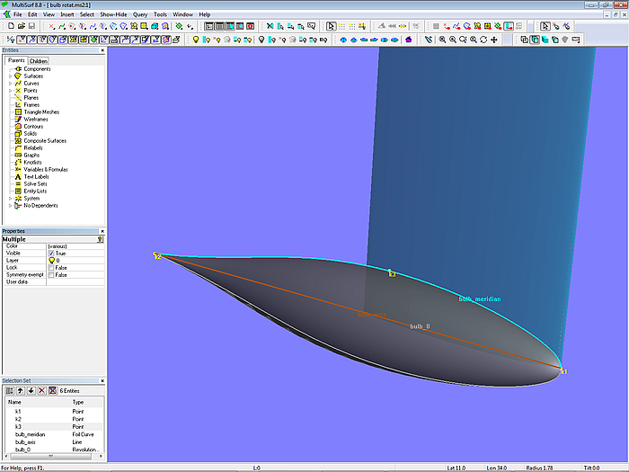
Model bulb_revolution_surface.ms2

 

For a gentle transition between keel fin and ballast bulb a Blend Surface is convenient.

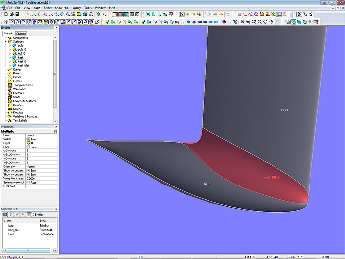
Model bulb_revolution_surface.ms2 - gradual transition from keel fin to ballast bulb by Blend Surface

 

Procedural Surface

The only freeform possibility in the previous method is the shaping of the meridian curve of the Revolution Surface. Its full cross sections are circles. Some more freeforming is offered by using the Procedural Surface entity to create the bulb. The model bulb_procedural_surface.ms2 shows an example.

 

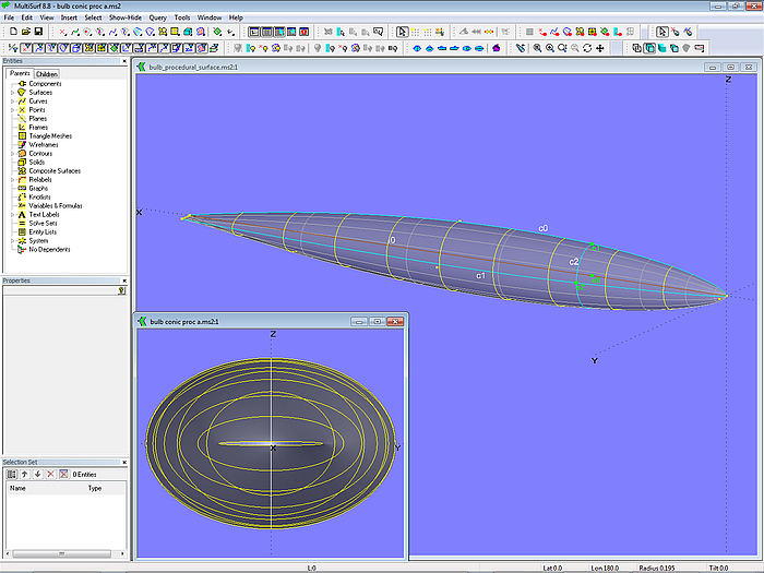
Model bulb_procedural_surface.ms2 – ballast bulb as Procedural Surface. The moving curve is an ellipse.

The outline in profile view is defined by the Foil Curve c0, while the maximum width in plan view is controled by the B-spline Curve c1. The moving curve is the Conic Section c2, with type set to “Ellipse”. The center of the ellipse is Bead e0, the Beads e1 and e2 define the end of the primary and the secondary axis. The angle range is from 0 to 180 degrees.

Driving point of the Procedural Surface construction is Bead e0 on Line l0. At the location of e0 the curves c0 and c1 are intersected in the XYZBeads e1 and e2, thus the parents for the ellipse c2 are defined. The surface is then created by moving the curve c2 along the axis line l0.

The cross sections of this bulb are of elliptical shape. In case the width of curve c1 near the tip of the bulb is similar to the height of curve c0 the sections will be more round. Again, the centroid of volume is on the axis line.

Note: Line l0 must be relabeled to make a correct tip of the bulb, its curve velocity must be zero here. The relabel used starts with two zero values: {0, 0, 1}, thus it produces zero velocity at the t=0 end of the line. (The velocity of a curve is the rate of change of distance (arc length) along the curve with respect to change in the t parameter.) Using a B-spline Curve with a double point at the t=0 end would be a workaround relabeling the line.

A variation of the foregoing bulb construction is shown in model bulb_procedural_surface_2.ms2. Here the bottom profile of the bulb is defined separately by a second Foil Curve. At the location of Bead e0 this Foil Curve c3 is cut in the XYZBead e3, which together with Beads e0 and e2 is used to create an ellipse (Conic c4) for the bottom of the bulb.

 

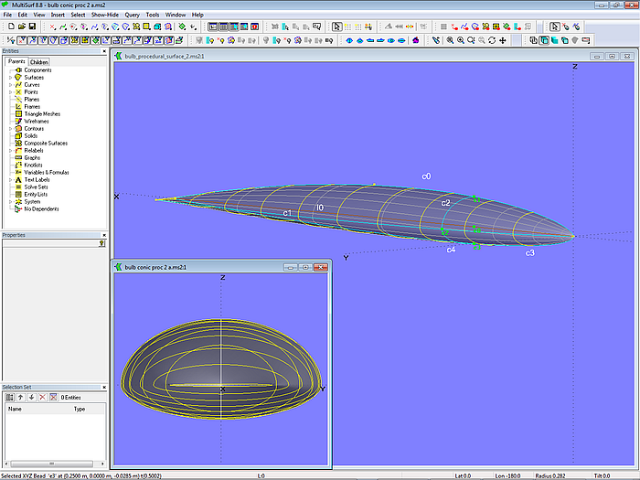
Model bulb_procedural_surface_2.ms2 - the moving curve is a PolyCurve combining an elliptical curve for the topside and a separate one for the bottom of the bulb.

Both Conic Section curves c2 and c4 are tied together by a PolyCurve which now becomes the moving curve of the Procedural Surface bulb. The angle range for both ellipses is from 0 to 90 degrees.

 

B-spline Lofted Surface

While in the previous examples the profile outline and the width of the bulb are free to the designer´s wishes, the cross sections are analytical curves – a circle with the Revolution Surface, an ellipse or a combination of two ellipses with the Procedural Surface.

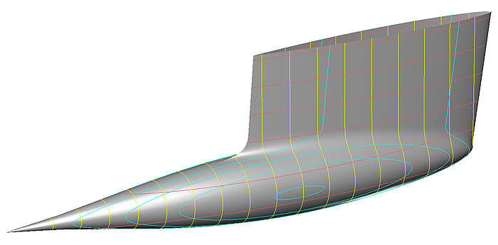
Full freedom to give the bulb any shape is provided using the B-spline Lofted Surface. An example shows model bulb_b-spline_lofted_surface.ms2. The model has 5 mcs. While mc1 at the tip is just a single point, mc2 to mc5 are B-spline Curves of degree = 3, all with 6 cps. The degree of the B-spline Lofted Surface is also 3.

 

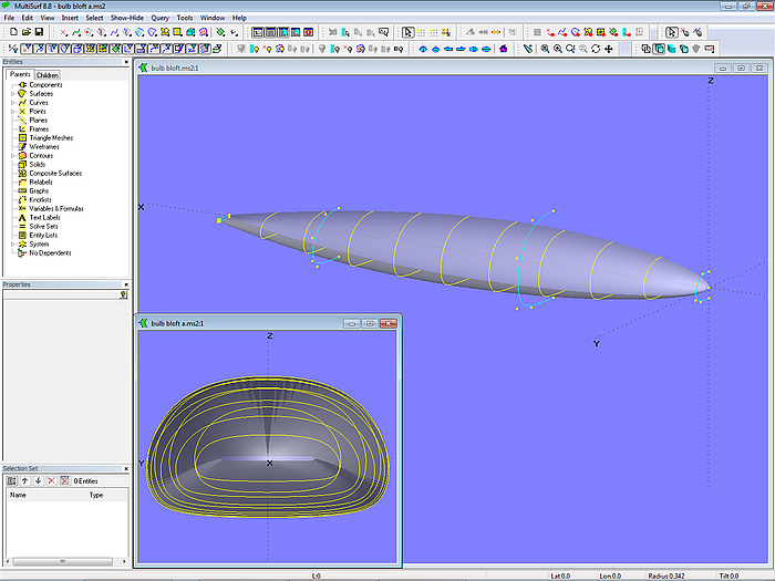
Model bulb_b-spline_lofted_surface.ms2

The mcs are running transversely; the dragging property for the cps is set accordingly to keep them in plane (same X-coordinate for cps). Of course there is no real need for this, but doing so the shape of the mcs will be closely related to the shape of the cross sections. So the process of forming will attain its end faster.

Profile outline as well as the cross section shape depend on the shape of the mcs. If the cross sections at the tip should be round, replace the B-spline Curve mc2 by a semicircle Arc.

 

B-spline Surface

Since the previous model shows a B-spline Lofted Surface on B-spline Curves of equal degree and same number of cps, the identical geometry can be created by a B-spline Surface using just the control points (model bulb_b-spline_surface.ms2).

 

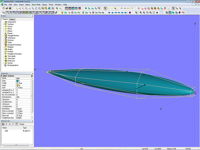
Model bulb_b-spline_surface.ms2 - B-spline Surface

Note, that the point for mc1 must be selected 6 times, as the number of cps in u-direction (transverse) is 6. Four entities (mc2 to mc5) are saved with this construction - however, it lacks the visual aid of the mcs in the B-spline Lofted Surface version.

 

Foil Lofted Surface

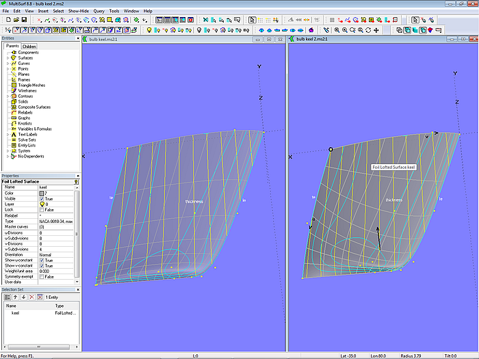
So far we considered bulbs as a separate element of the keel appendage, that is: keel = fin + bulb. However, if a more traditional keel planform is intended, then the increase of the thickness ratio towards the keel tip will also lower the center of gravity of the ballast. Model keel_foil_lofted_surface.ms2 shows an example.

 

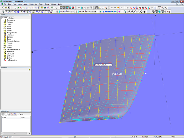
Model keel_foil_lofted_surface.ms2 - Foil Lofted Surface defined by 3 mcs: trailing edge, thickness and leading edge

The construction is simple. Three mcs control the Foil Lofted Surface – trailing edge, thickness and leading edge. Due to their ease to form (“cooked spagetti”) it is convenient to use B-spline Curves of equal degree and same number of cps. What means, that the most complex curve determines the number of cps on all mcs. In the example under discussion the trailing edge could easily be done with just 3 points. But since the thickness curve requires 5 cps, the trailing edge must be defined by 5 cps too.

Attention has to be paid to the requirement that corresponding cps must have equal Z-coordinates. Otherwise the t-parameter distribution of the mcs will be different what results in distorted u-constant parameter curves of the Foil Lofted Surface with severe detrimental effects to its fairness. (See also the article “Modeling a Rudder in MultiSurf”.)

 

Effect of unsimilar t-parameter distribution. Right: the trailing edge curve is defined by 3 points, while thickness and leading edge curves are supported by 5 points.

 

If these requirements are considered too restrictive the construction by a Procedural Surface will offer flexibility. The curve type for the mcs of trailing and leading edge and thickness can then be chosen to suit best one´s needs. For example, a Line or C-spline Curve for the trailing edge, and B-spline Curves for leading edge and thickness curves, both of different degree and divers number of cps.

 

Model keel_procedural_surface.ms2 – the use of a Procedural Surface avoids a distorted net of parameter curves. The trailing edge is a C-spline Curve with 3 cps, the moving curve is a Foil Curve.

 

Volume and centroid

There are three possibilities to show volume and its centroid while modeling.

• Hydrostatics
• Hydrostatic Reals
• Solid

 

1. Hydrostatics

–  Create a Contours entity of closely spaced stations
–  Open an Offsets View window
–  Select Tools/ Hydrostatics

The image below shows a convenient arrangement of the various windows on the screen (model keel_hydrostatics.ms2). When the Hydrostatics window is open the Offsets View window can also be minimized to get it out of way completely.

A disadvantage in the author´s view is the display of the station contours in Wireframe or Shaded View. It turns away the eye from the objects which controls the shape. Hiding the contours is not feasible, the Offsets View will be empty as well as the Hydrostatics window.

 

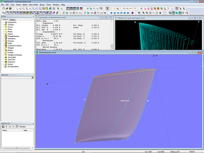
Model keel_hydrostatics.ms2 - screen arrangement for modeling and checking volume data simultaneously

 

2. Hydrostatic Reals

Hydrostatic Reals offer a second path to show volume and centroid data during the modeling process. Hydrostatic Reals are a group of Formula functions similar to functions like Angle or Area.

Model keel_hydro_reals.ms2 demonstrates the method. Because the station contours must start and end on centerplane the top of the keel is closed by a Ruled Surface.

 

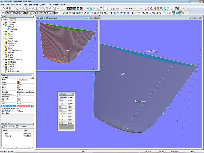
Model keel_hydro_reals.ms2 – display of volume and centroid while modeling. Upper left window: the keel top is closed by a Ruled Surface because station contours must start and end on centerplane.

The result of the calculation is displayed via Tools/ Real Values or with the help of Text Labels. The contours, on which the calculation is based, can be hidden.

 

3. Solid

Tools/ Mass Properties displays point coordinates, length of a curve, area of a surface and so on. It also shows volume and centroid of the entity Solid. Model keel_solid.ms2 explains this method.

In order to create a solid the keel surface is mirrored against the centerplane (Y=0 plane), then a Ruled Solid is spanned between keel surface and its mirror image. When the solid is visible its properties are listed in the Mass Properties window.

A direct display of volume and centroid can be achieved by using the Formula entity. The solid can then be hidden.

 

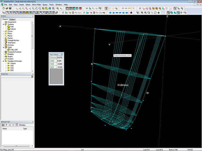
Model keel_solid.ms2 - display of data for volume and centroid of the keel solid

When the keel surface is edited, its mirror image and the solid gets updated too, and so will the display of volume and centroid.

Of course, further data like wetted surface area, lateral area and centroid can also be exposed using functions offered by the Formula entity.

====================================================================================