How to Create Computing MultiSurf Models
Variables, Formulas and Functions
by Reinhard Siegel
Contents
Basic Concept – Variables, Formulas, Functions
- Variables
- Formulas
- Functions
Application Examples of Variables and Formulas
- I-Beam
- Main Dimensions
- Sailplan
- Lateralplan
Advanced Application of Variables and Formulas
- Hydrostatic Reals
- Flotation Waterline Upright – Balance
- Flotation Waterline at Heel – Balance
- Yacht Hull Resistance
- On the Layout of Planking
- Modeling the Hull Measurement Rules of Square Metre Yachts
Mathematical Functions Available in MultiSurf
Introduction
There are two ways to specify a real number in the definition of an object: with a constant value or a real entity. Variables and Formulas are example of real entities. A Variable carries a value that lies within a specified range. A Formula involves an expression made of real entities, constants, operators and Functions. Variables and Formulas can be parents of all objects depending on a real value. Therefore they can be supports of points (as coordinates, offsets, angles, t-, u- and v-parameter), curves and surfaces (via knot lists and weights), etc.
What are the advantages of Variables and Formulas?
With Variables and Formulas simpler, clearer models can be created. Models can be changed immediately, you do not have to search for the point that controls a certain part of the construction, one can directly select the variable in the Entities manager and then change its value. Example I-beam: for the given basic geometry just 4 measurements determine the shape. Using Variables and Formulas the coordinates of necessary auxiliary points do not need be individually constructed, their coordinates can be determined by calculation.
Variables and Formulas can be used to create models that carry out calculations: main dimensions, area sizes and center of gravity, rating rule measurements, floating position, hydrostatic characteristics, hydrodynamic resistance and so on. In this way, a model can provide additional information to the designer about itself, always updated immediately upon a change of model shape.
Variables and formulas expand the functionality of MultiSurf enormously. MultiSurf is limitless.
Abbreviations used:
cp: control point (support point)
mc: master curve = support curve
cp1, cp2, ...: denotes 1st, 2nd, ... point in the list of supports of a curve. It is not an actual entity name.
mc1, mc2, ...: denotes 1st, 2nd, ... curve in the list of supports of a surface. It is not an actual entity name.
In the following the terms used for point, curve and surface types are those of MultiSurf. This may serve the understanding and traceability.
Basic Concept – Variables, Formulas, Functions
Variables
When a standard 3D point in MultiSurf is created, its coordinates dx, dy and dz must be entered. Typically a concrete number, say 1.2345, is used to specify the value of a coordinate. On the other hand, instead a number one can use a Variable, a symbol for any element of a given quantity.
Let us consider the model box-1.ms2, a box shaped body.
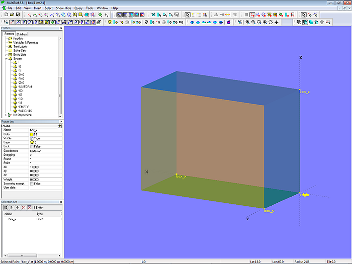
Model box-1.ms2 – squared box
Its length is determined by Point box_x, the breadth by Point box_y and its height by Point box_z. The dx, dy, dz coordinate values are (1;0;0), (0;0;0.5) and (0;0;0.75). Dragging any of these points will change the corresponding dimensions of the box.
Model box-2.ms2 looks identical. However, now the dimensions are determined with the 3 Variables length, breadth and height. For example, the dx-coordinate of the point box_x is not set to the numeric value 1, but the Variable entity length is entered here.
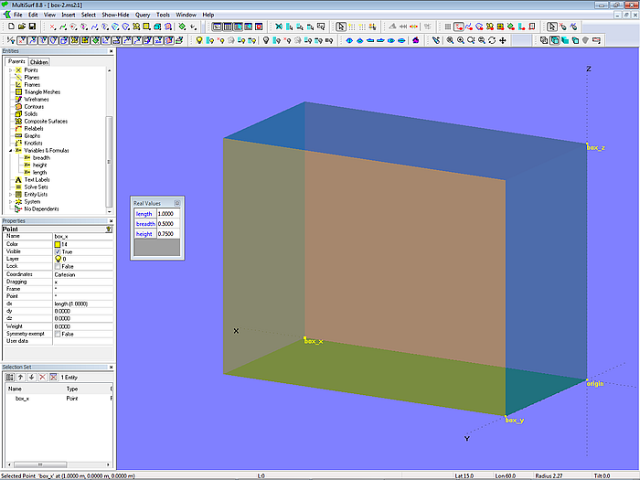
Modell box-2.ms2 – variables control the dimensions of the box.
To display all Variables in a model, you can select "Tools/ Real Values" from the main menu or simply press the "V" key on the keyboard. The current value of Variables can be changed in the appearing "Real Values" dialog box. Or you select them in the Enities manager and then edit them in the Properties manager.
Contrary to points, which can only be moved manually on the screen when they are visible, objects defined with Variables can be hidden. For example, simply change the value in the "Real Values" window and the model is updated.
Variables can be parents of all objects that depend on a real value. Therefore, they can be parents of points (as coordinates, offsets, angles, t-, u- and v-parameter values), as well as curves and surfaces (via knotlists and weights).
In a geometry where the general shape is fixed, but dimensions are still open, Variables can advantageously be used. For example, for the cross-sectional dimensions of longitudinal frames; the height and width of a foot-rail; the radius of fillets between surfaces in the cockpit, etc.
Formulas
A Variable is assigned a specific value (box-2.ms2). If, for example, the length of our box should be always the twofold of its height, this condition can not be implemented into the model by a Variable. Instead the object Formula must be used. Formulas provide the result of a calculation with constants, variables with operators (+, -, * etc.) and functions.
In the model box-3.ms2 this is illustrated.
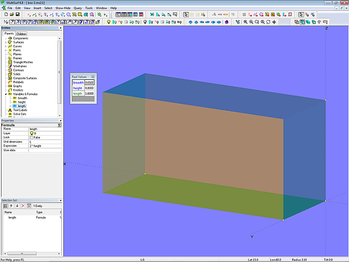
Model box-3.ms2 –the Formula length controls, that the dimension in X-direction is twice the height of the box.
The "Real Values" dialog box displays the names of Variables and Formuals in different colors. Only the values of Variables can be changed here. For Formulas the result of the calculation expression is displayed.
Model box-3.ms2 is just a simple calculating model. Using Variables and Formulas much complexer models can be created, for example to compute class rule measurements, position of center of effort, floating position, etc.
Functions
An important component of Formulas are Functions which can be used in the computational expression. With Functions, the dx, dy, dz coordinates of a point can be determined, or the distance between 2 points, mathematical operations can be executed like raising a number to a higher power, etc. Or, as demonstrated in model area-1.ms2, the size and center of a surface can be derived.
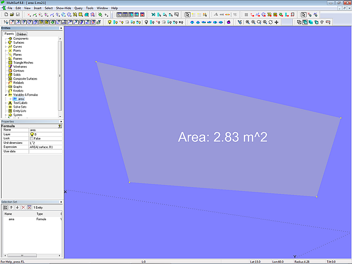
Model area-1.ms2 – application of the function AREA
When the shape of the surface is changed by moving its control points, the area size is recalculated and displayed by a Text Label.
Often used Functions
Often used functions for use in the expression of Formulas are the following ones:
- XPOS, YPOS, ZPOS: returns the XYZ position of a point
- TPOS returns the t position of a point
- ARCLEN: return the girth length between two curve points (rings)
- DIST: returns the distance between two points
- AREA: returns the area of a surface
- CENTROID: returns the XYZ coordinates of center of area
- HYDRO: returns hydrostatic values (for fixed position and in combination with the entity Solve Set also for free flotation)
The complete set of Functions available is listed at the end of this tutorial.
Function DIST
Let us consider a simple example: the model wl_length.ms2.
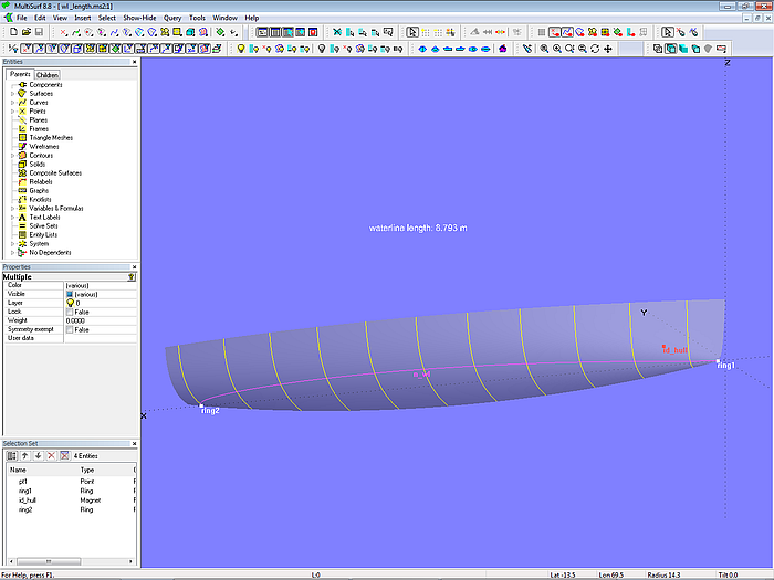
Model wl_length.ms2 - calculation of waterline length by Formula
The model holds the surface hull. We want to measure its waterline length.
- Create Magnet id_hull in the bow area.
- Intersect the hull by the *Z=0 plane. This is the Intersection Snake n_wl.
- Put ring1 at the start of the intersection snake.
- Put ring2 at the end of the intersection snake.
- Create the Formula wl_length using this expression:
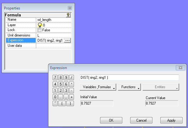
Expression used in Formula wl_length to calculate the distance between the waterline ends
The function DIST is used to calculate the distance between the two rings. (Please note, that the use of the DIST function implies that both rings have coordinates Y = 0 and Z = 0.)
In order to display the result of our calculation (i. e. the value of Variables and Formulas) we have two options:
- Real Values
- Text Label
For display of Real Values use in the Tools menu the entry “Real Values” or press the shortcut letter key “V”.
To present the values of Variables and Formuals by the entity Text Label follow these steps:
- Create a point serving as the handle of the Text Label (here this is Point pt1)
- Insert the Text Label entity. Note, that the property “Legend” provides input for a discription as well as for the formating of the displayed value.
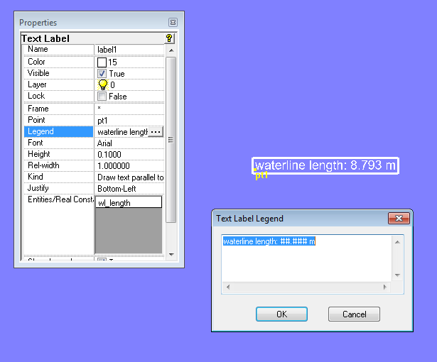
Display of real values of Variables and Formulas via Text Label
Function TPOS, XPOS, YPOS, ZPOS
Model positions.ms2 illustrates how to find the XYZ-coordinates of a point and the t-parameter value of a bead or ring. The Formula t_e1 returns the t-parameter of Bead e1; the expression simply reads: TPOS (e1). The Formula x_e1 returns the X-coordinate of Bead e1; its expression is: XPOS (e1). Likewise the Function for the Y- and Z-coordinates are YPOS and ZPOS.
Function AREA, CENTROID
In model area-2.ms2 – similar to the previous example – the size of the surface area is calculated by means of the AREA function. In addition the CENTROID function calculates the coordinates of the center of gravity. The point CE is defined with these.
Model area-2.ms2 – application of the functions AREA and CENTROID
The Formula area uses in its expression the Function AREA (surface, use_sym). It needs two arguments: first, the name of the surface entity and second, the figure 0 or1, which controls the use of symmetry (0 = no symmetry; 1 = use symmetry). Here the expression for the Formula area reads: AREA ( s0, 0 ).
The Function for the centroid of the surface is: CENTROID (entity, use_sym (0 or 1), index (1-3, for X,Y,Z coordinate). It needs three arguments. Thus the expression for the formulas used to define Point ce reads: cex: CENTROID( s0, 0, 1 ); cey: CENTROID( s0, 0, 2 ); cez: CENTROID( s0, 0, 3 ).
Function ARCLEN
In model arc_length.ms2 an example is given for the Function ARCLEN. It requires 3 arguments: curve name and two t-positions. The Formula length_01_05 calculates the arc length of curve c0 between t = 0.1 and t = 0.5. Thus the expression of length_01_05 reads: ARCLEN( c0, 0.1, 0.5 ).
If we want to know the arc length between two beads or rings on a curve or snake, then the Function TPOS can be used. TPOS returns the t-parameter value of a bead or ring.
In model arc_length.ms2 the beads e1 and e2 lay on curve c0. The Formula length_e1_e2 calculates the arc length between both beads. The expression of length_e1_e2 is: ARCLEN( c0, TPOS(e1), TPOS(e2)).
Application Examples of Variables and Formulas
In the following models extensive use is made of Variables and Formulas in order to build-in flexibility and derive information on the geometry.
I-Beam
Model I-beam.ms2 is included in the “Examples” folder of MultiSurf. It shows how the corner point coordinates of the web and the flanges are determined from the height, width and thickness of an I-beam. The Formulas d1, d2 and d3 only use simple arithmetics in the respective computational expression.
Model I-beam.ms2 – from the MultiSurf Examples folder. 4 variables define the shape.
Main Dimensions
The model main_dimensions.ms2 determines the main dimensions of a boat hull. Essentially, the Functions XPOS, YPOS and ZPOS are used in the formulas to determine the XYZ coordinates of points. For example, the overall length, the length in the waterline, the front or rear overhang, etc.
Model main_dimensions.ms2
To find the location of the maximum width of deck and waterline Proximity Rings are used – independently MultiSurf searches the curve point with the greatest distance from the midship level.
A series of text labels display the results.
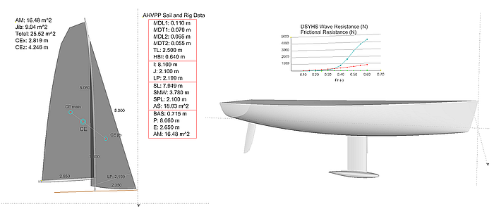
Sailplan
The model sailplan.ms2 shows a sailplan, the geometry of which is defined by dimensions of rig and sails. Formulas are used to calculate area and centroid for mainsail and foresail as well as for both.
Model sailplan.ms2 – in the Real Values windows rig and sail dimensions can be edited.
There are the Entity Lists edit_rig_dimensions and edit_sail_dimensions which hold the corresponding variables for rig and sails. Select a list, then press the key “V” or select main menu/ Tools/ Real Values to open the Real Values window. Here new values can be entered. For example, change the length of the jib foot to 3.2 m and the sailplan will change to the new setting. Sail areas, total area, center of effort etc. are updated accordingly, providing the designer with valuable information.
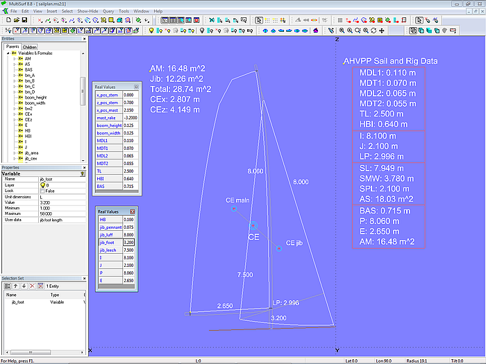
Model sailplan.ms2 - foot length of foresail increased
Lateralplan
The model lateralplan.ms2 computes design data of the lateral plan of the underwater body of a sailboat. The surface portions of hull and rudder below the waterline are first created with SubSurfaces, which are then projected onto the midship plane by Projected Surfaces. The keel can be projected directly.
Then the individual areas and centroids as well as their sum are determined analogously to the sailplan model. Small circles around points with their coordinates according to the Formula values illustrate the center of efforts.
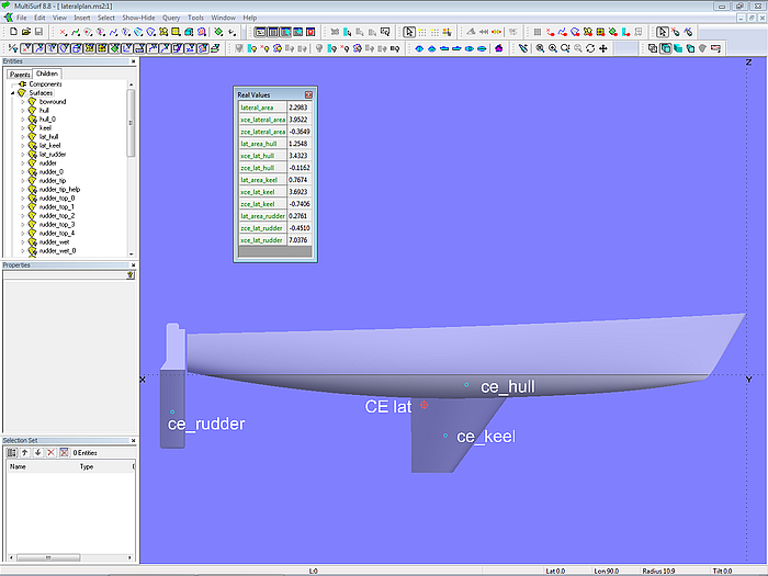
Model lateralplan.ms2 – calculation of lateral areas and centroids of hull, keel and rudder
Advanced Application of Variables and Formulas
Hydrostatic Reals
Among the variables and formulas provided by MultiSurf there is a special type called Hydrostatic Real. By use of Hydrostatic Reals it is possible to display hydrostatic properties for given sink, trim and heel while editing the hull shape. Also Hydrostatic Reals allow to determine the flotation waterline for given weight and center of gravity. This is convenient for valuation of the shape of the waterlines at various loading conditions. Also the actual waterline under heel can be seen, what is practical to check for transom immersion.
The parents for a Hydrostatic Real are:
- Sp. Gravity
- Zcg
- Sink
- Trim
- Heel
- Type
- Contour List
The first 5 parents are the same you would enter when calculating hydrostatics byTools/ Hydrostatics.
Type specifies which hydrostatic property the Hydrostatic Real will show. There is a total of 29 types, covering all the hydrostatic properties of Tools/ Hydrostatics.
Contour List specifies the name of an Entitiy List, which contains the names of the cross section contours used to calculate the Hydrostatic Reals. Note, that those contours can be hidden – this is very convenient to avoid a cluttered screen.
In the model Hydro_reals_example-1.ms2 there is the C-spline Lofted Surface hull_0 and the flush Ruled Surface deck_0 (to get closed transverse contours). Parent for the Contour List is the Entity List Hydro_contours, which holds the cross section contours hydro_stations1, hydro_stations2 and hydro_stations3, cutting hull_0 and deck_0.
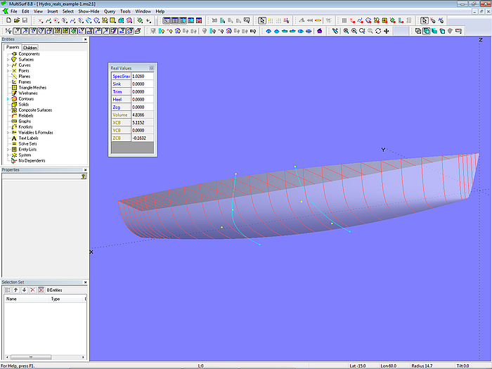
Model Hydro_reals_example-1.ms2 - calculation of hydrostatic data by the special formula type Hydrostatic Reals
The reason for using a group of 3 cross section contours is to improve the calculation accuracy where the hull shape changes faster. Very dense station spacing will delay program response.
The model provides Hydrostatic Reals for Volume, XCB, YCB, ZCB. When the model is open, press the key “V” or select main menu/ Tools/ Real Values. Change a master curve - the Real Values window immediately shows the new values.
Click in the Real Values window on Sink and change it - again, the values are updated.
The model Hydro_real_example-3.ms2 provides all available Hydrostatic Reals.
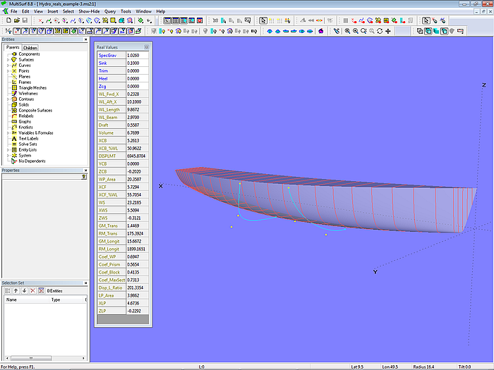
Model Hydro_reals_example-3.ms2
So far to this introduction how to use Hydrostatic Reals for the calculation of hydrostatic properties.
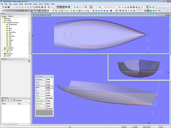
Flotation Waterline Upright – Balanced
In the previous model hydrostatics are calculated for a fixed position of the boat in the water. By use of the Entity Solve Set it is possible with Hydrostatic Reals to answer the question, how the boat will float for a given weight and a given center of gravity. The Solve Set iterates sink and trim until there is an equilibrium between weight and buoyancy forces and moments.
The model Hydro_free_floating.ms2 is basically similar to the example above. Again there is the C-spline Lofted Surface hull_0 and the flush Ruled Surface deck_0, cutted by the Contours hydro_stations1, hydro_stations2 and hydro_stations3.
Parent of the Contour List is the Entity List Hydro_contours which holds the Contours hydro_stations1, hydro_stations2 and hydro_stations3, cutting hull_0 and deck_0.
The Point mass_boat represents the weight of the boat and its center of gravity. Let us assume, that the weight estimation of the finished boat amounts to 5200 kg, and its center is at Xcg = 5.25 m. So the property Weight of Point mass_boat is given the value 5200 (kg). For the longitudinal position (coordinate dx of mass_boat) the Variable Xcg is created, its value is set to 5.25 (m).
Further there is the Roll-Pitch-Yaw-Frame F_float, which is the coordinate system of the boat in balanced and trim free condition. The hull surface hull_0 is copied into this frame to show the free floating hull (Copy Surfaces hull_float_stb and hull_float_ps).
Model Hydro_free_floating.ms2 - balancing of weight and buoyancy forces and moments
When the model is open, show the “Real Values” window (letter key “V” or main menu/ Tools/ Real Values). In the Entities manager open the category Solve Sets and select ss1. A look to the Properties manager reveals, that at current Type is set to "Dormant". This means there is no balancing of weight and buoyancy.
In the upright position (Heel = 0 ) with Sink = 0 and Trim = 0 the volume is 4.84 m^3, displacement is 4961 kg and XCB is at 5.12 m.
However, the estimated boat weight is 5200 kg and Xcg is at 5.25 m. So what then is the flotation for this situation?
To find the flotation waterline for this weight condition set the Solve Set ss1 to “Active”. Sink and trim are now adjusted to make the displacement equal to the weight of the boat as well as XCB and Xcg above each other vertical to the waterplane. The result is a Sink of -0.024 m and a Trim of 0.37 degrees. Now you have a clear information how much the deviation in Sink and Trim is between actual and wanted displacement. Now you as the designer can answer the question: stop with the hull modeling or make appropriate changes.
Flotation Waterline at Heel – Balanced
A related problem is to determine the design waterline at heel. May the purpose be the judgement of the asymmetric shape of the waterline, may it be the question, whether the transom is still free of the waterplane or already immersed. Heeling with fixed sink and trim will give wrong results, as the volume will increase. The boat must by free floating when heeled to get realistic answers.
The model Hydro_free_floating.ms2 is already set-up for the answer. Just enter a heel angle, say 15 degrees. In the Entities manager open the category “Variables and Formulas”, select the Variable Heel and then in the Properties manager enter the wanted value. Or set the heel angle quickly via the “Real Values” window. The active Solve Set ss1 will adjust Sink and Trim according to the weight conditions defined by the Point mass_boat.
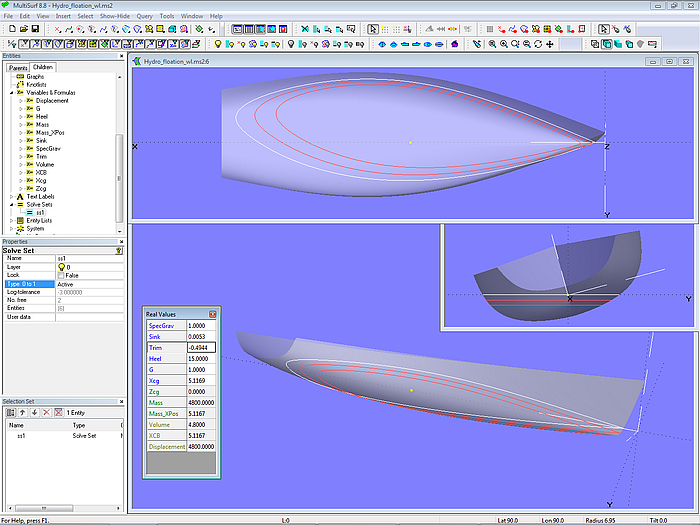
Model Hydro_flotation.ms2 – free floating at heel
So far to Hydrostatic Reals and how they can provide useful information in the hull design process.
Yacht Hull Resistance
Via Variables and Formulas the prediction of hydrodynamic quantities can be implemented in a hull model. For example, for sailing boats there are the results of the famous research work well known as the Delft Systematic Yacht Hull Series (DSYHS).
The model DSYHS.ms2 computes wave resistance and frictional resistance according to DSYHS equations presented in the book Aero-Hydrodynamics and the Performance of Sailing Yachts (Fabio Fossati; Adlard Coles Nautical, London, 2009).
The expression used for wave resistance is (page 24):
Rw LCB V^(2/3) BWL V^(1/3) LCB
----------- = a0 + ( a1 * ------- + a2 * Cp + a3 * ----------- + a4 * -------- ) * ----------- + ( a5 * -------- +
V * ρ * g LCF AWP LWL LWL LCF
BWL V^(1/3)
a6 * -------- + a7 *Cm ) * -----------
Tc LWL
where
- Rw is the wave resistance (N)
- LWL is the theoretical waterline length (m)
- BWL is the theoretical waterline beam (m)
- Cp is the prismatic coefficient
- V is the canoe body volume (m^3)
- LCB is the longitudinal center of buoyancy position from the forward perpendicular (m)
- LCF is the longitudinal center of flotation position from the forward perpendicular (m)
- AWP is the waterplane area (m^2)
- Tc is the canoe body draft (m)
- Cm is the midship section coefficient
- g is acceleration of gravity (m/s^2)
- ρ is the density of water (kg/m^3)
- a0 ... a7 coefficients, function of Froude number (Table 2.5, page 24)
The expression used for the frictional resistance is (page 14):
Rf = ½ * ρ * v^2 * Cf * AW
where:
- Rf is the frictional resistance
- ρ is the density of water (kg/m^3)
- v is the boat speed (m/s)
- Cf is the skin friction coefficient
- AW is the wetted surface (m^2)
The formula for the skin friction coefficient is:
0.075
Cf = ----------------------------------------------
(lg(588000 * LWL * v ) – 2) ^2
It is derived from the ITTC 57 formula using 70% of the waterline length for the calculation of the Reynolds number.
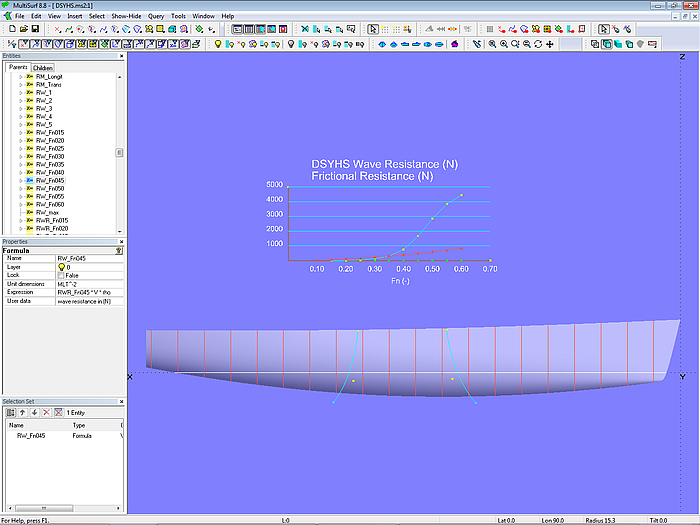
Model DSYHS.ms2 – implementation of Delft Systematic Yacht Hull Series equations for wave and frictional resistance
The hydrostatic values required for the calculation of the formulas are determined in the manner explained above with Hydrostatic Reals. The wave resistance is calculated for 10 Froude numbers in the range from 0.15 to 0.60 with the respective coefficients a0 - a7. The friction resistance is determined for boat speeds according to these Froude numbers.
The Entity Lists frictional_resistance, wave resistance and velocities are there to show the corresponding numerical values - select the Entity List, then press the "V" key or select main menu/ Tools/ Real Values.
The results are displayed in a diagram. To compare with hull form changes, one can use TempCopy to save current graphs from being overwritten (press key "w" or main menu/ Tools/ Commmand Window). TempCopy wireframes can also be stored as permanent 3DA wireframes.
On the Layout of Planking
The run of planks on a classic boat hull must look harmonious. In order to get there, this principle applies: between sheerstrake and garboard strake all planks should have the same width at the same mould. The following is a description of how to define the planking process using MultiSurf.
Hull
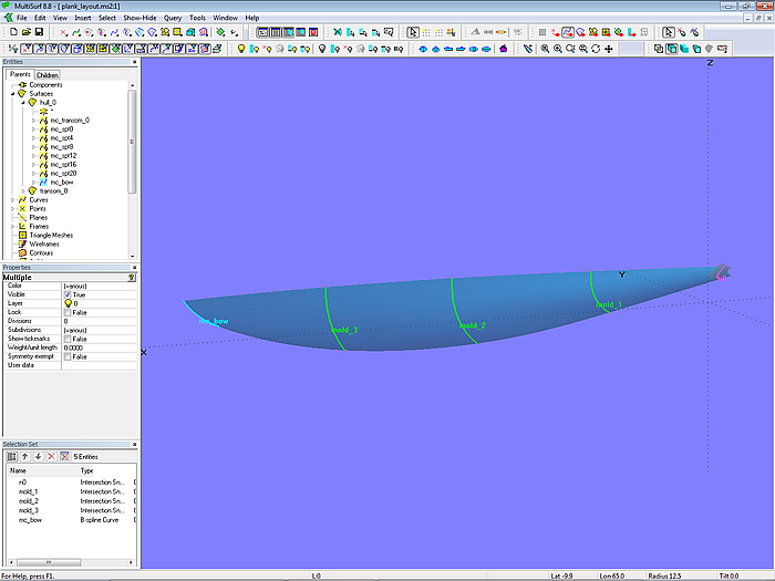
The example here is the model plank_layout-1.ms2. It holds just those objects which are required to explain a method of layout the planking of a wooden boat hull.
The hull is a standard C-spline Lofted Surface on B-spline master curves.
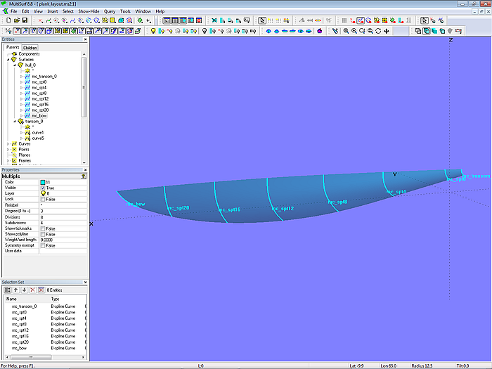
Model plank_layout-1.ms2 – C-spline Lofted Surface on B-spline master curves
Why so simple?
Why is there no keel appendage?
Why the assumption, that the planks end at stem, fairbody and transom beam and not on rabbet curves?
This here is an example. The more of those details, the more complex the model and the view on the screen, the less the understanding of the subject in question.
The shape of the planks, that is, the run of their longitudinal edges or seams are defined in two steps. First, C-spline Curves are created as guides for the seams. Second, the C-spline Curves are projected onto the hull surface as Projected Snakes to create the actual plank edges.
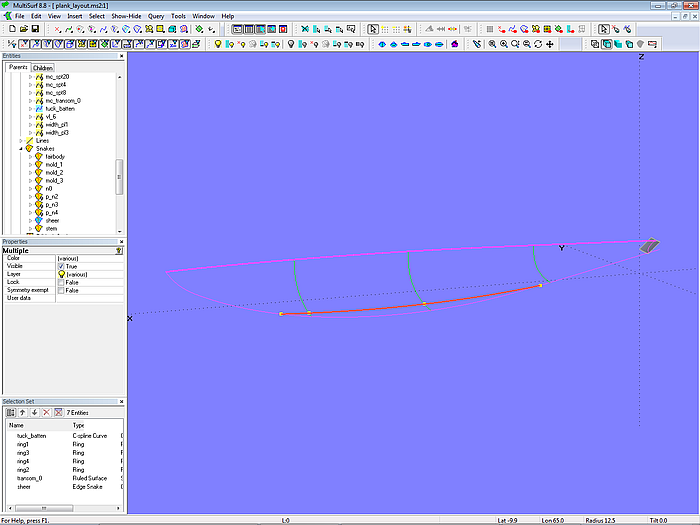
Molds for plank seam definition
The seam guides are passing through a series of points on hull molds. Here transverse molds in the middle of the hull are used; this are Intersection Snakes. The aft mold is the intersection of hull and transom. Some of the seam guide curves start on rings on the transom beam and end on the forward fairbody or stem.
Why 3 interior molds? (For the 75 sqm boat 10 molds were used.)
This is an example. The more molds, the more things one must pay attention to. Understanding the principle idea is the goal.
Model plank_layout-1.ms2 - support curves for the plank seam guides (these are no hull master curves)
The tuck batten
In this example we only deal with the region for the planks between the sheer and the tuck batten curve. This curve devides the planks of the hull side and the planks of the keel side. It starts where the sternpost touches the transom beam. And ends somewhere at the forefoot. It is a geodesic curve on the hull, the shortest path on the surface, like a string pulled tight between its end points on the hull.
Model plank_layout-1.ms2 - planking region between sheer and tuck batten
In the example the tuck batten is a C-spline Curve supported by rings on the fairbody and the molds.
Plank layout – general rule
The general rule for plank layout is: at each mold the girth length is divided into equal plank widths.
Thus we need to measure the girth of a mold from its upper end to the location of the tuck batten. This is easily done via Tools/ Measure/ Distance (or the corresponding toolbar button).
Let us take for example mold_2. Select Ring ring6 (top end) and Ring ring4 (tuck batten), then select Tools/ Measure/ Distance. Since the measurement is done for two Ring entities on the same snake, the distance report also shows the Arc length between the points.
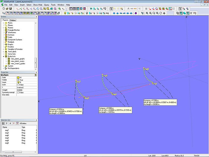
Model plank_layout-1.ms2 - distance reports for 3 molds
At mold_2 the Arc length is 1.07 m. If we want 11 planks of equal width, each is 0.097 m. Consequently we put on mold_2 10 Arc-length Rings each 0.097 m apart from the previous one.
At mold_3 the girth is 1.008 m, resulting in a width of 0.091 m for 11 planks.
Model plank_layout-1.ms2 - plank seam guides
Together with rings on stem, transom beam and fairbody those Arc-length Rings on the molds provide the control points for the seam curves.
Please note, that at mold_1 the situation is different, the tuck batten starts forward of this station. Only 10 planks of equal width can be attached and where should the bottom ring (ring5) for the girth measurement be positioned? Since the start point of the seam curve (ring9 on the fairbody curve) is close to mold_1, its location must also be carefully set to achieve a sweet running seam curve (C-spline Curve c_n11).
Also the plank widths along the stem end and transom beam end must change in a harmonious fashion. Checking carefully in 3D by rotating the model and looking along the seam curves is at least as convenient as establishing the lay of the planks on the full scale hull in the workshop.
Our example here holds the assumption, that the sheerstrake is not wider than the planks further below. In case a wider sheerstrake is desired, for example to compensate for a covering guard-rail, define this plank first, then start the girth measurements from its lower edge.
As said, this is an example. The more molds, the more things one must pay attention to. Understanding the principle idea is the goal.
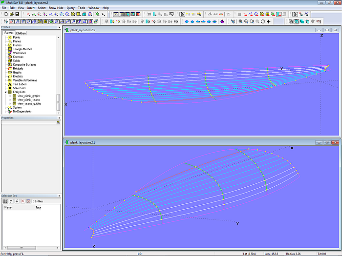
Graph of plank width
In order to make sure that the planks taper in a fair way a graph of the plank width is helpful. The model plank_layout-1.ms2 shows graphs for plank no.1 and no.3.
The construction is not that much complex, it uses Copy Beads, Copy Curves and Intersection Beads (Mirror is a point, thus a sphere is the cutting entity) to transfer plank width at 0, 20, 40, 60, 89 and 100 percent of the plank length to a grid of lines of equal proportional distance.
The Entity List view_plank_graphs holds parents and children of the graphs. They will automatically update if underlying objects are changed.
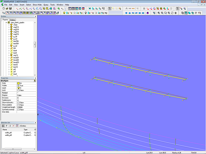
Model plank_layout-1.ms2 - graphs of plank width
Calculation of plank width by variables and formulas
The model should be enhanced to avoid tedious editing. For example, when the shape of the tuck batten is changed, the mold girths will also change. But there is no automatic adaption of the plank width.
In model plank_layout-2.ms2 this is done with the help of variables, functions and formulas. One must specify just the number of planks at a certain mold, and the model will position automatically all those Arc-length Rings closer or further apart.
The expressions in the formulas are simple. For example, the Formula al_mold_1 returns the arc-length between ring8 and ring5 on mold_1: al_mold_1 = ARCLEN( mold_1, TPOS( ring8 ), TPOS( ring5 )).
The Variable n_mold_1 specifies the number of planks. Thus the Formula d_mold_1 for the plank width at mold_1 is just: d_mold_1 = al_mold_1 / n_mold_1.
Whatever is now changed, be it the hull shape itself or the run of the tuck batten, the plank width is automatically adjusted.
Modeling the Hull Measurement Rules of Square Metre Yachts by Variables and Formulas
Introduction
The design of a yacht in accordance with specific class regulations requires the permanent comparison of hull dimensions against rule measurements. The functionality "Distance Mode" (Tools/ Measure/ Distance) provides a dynamic display of the distance between two points (also arc length distance, in case the points lie on the same curve/snake). A series of distance reports can easily be created to show hull particulars.
However, distance reports are not persistent between MultiSurf sessions (also are not included in Undo/Redo sequences). Often class rules require some further mathematical operations of measured values. Thus the application of variables and formulas is a more powerful way to produce class rule measurements for use in the design process.
The implementation of a measurement rule in a MultiSurf model is shown here by means of the rules for the square metre yachts (skerry cruisers).
Rules for square metre yachts
Basis for the hull regulations is a table of hull particulars of an ideal square metre yacht. If certain measurements exceed the ideal ones, displacement, mean breadth, freeboard and length of keel are to be increased.
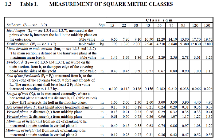
Table I: ideal hull particulars (taken from "Rules for skerry cruisers (square metre yachts)", SSKF, 2013)
Measurements are taken at a variety of horizontal and transverse sections.
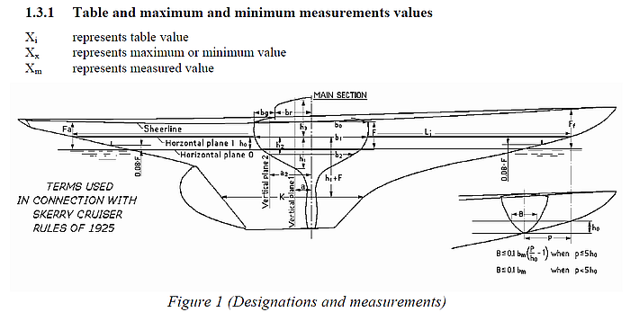
Definition of horizontal and transverse measurement sections (taken from "Rules for skerry cruisers (square metre yachts)", SSKF, 2013)
Example: 15 square metre yacht
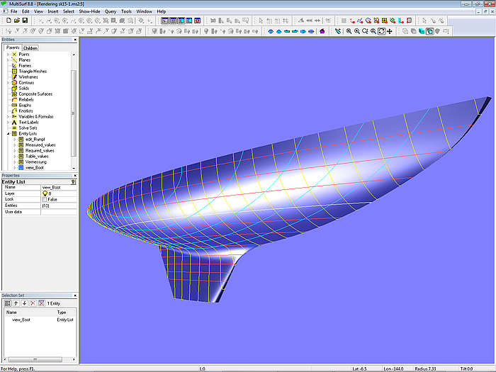
As an example we will consider the hull model of a 15 square metre yacht (sk15-1.ms2). By no means it is intended to create a complete model with deck, transom, rudder and so on. It is also not about a hull shape of specific proportions except that it fits to the class rules.
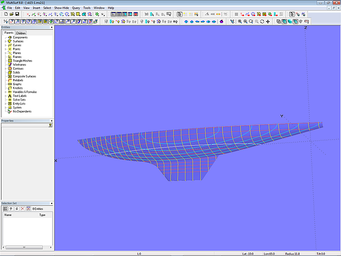
Model sk15-1.ms2 - 15 square metre yacht hull
The boat is composed of 3 surfaces: the C-spline Lofted Surface hull_0 (canoe body), the B-spline Lofted Surface keel_0 (basis keel) and the Blend Surf keel_fillet (transition from canoe body into keel).
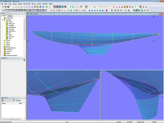
Model sk15-1.ms2 - canoe body, keel basis and fillet
The canoe body is defined by 8 mcs, each a B-spline Curve of degree 3 with 6 cps. Vertex curves (C-spline Curves which connect corresponding cps) serve as guides for fairing. The keel basis is supported by 3 B-splines with 6 cps each, running in waterline direction. The keel fillet is supported by B-spline Snakes, each controled by 6 magnets.
There are several Entity Lists. Select one, then use "Show Parents" to display their members. For example, the Entity List edit_hull 0 holds all entities for shaping the hull.
The Entity List measurements contains the measurement data. Its display is by Text Labels. The group "Table Values" holds the data according to Table I. The table values are implemented by Variables.
The group "Measured Values" lists the result of measurements at the various locations. Formulas are used for calculation.
The group "Required Values" shows the increased dimensions if length exceeds the ideal length Li.
There are also separate entity lists for these data, defined by variables or derived from formulas. This allows their display via Tools/ Real Values or the shortcut key "V" in separate windows.
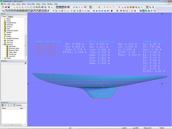
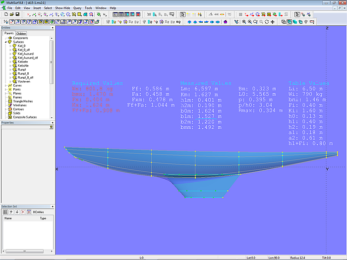
Model sk15-1.ms2 - measurement data and defining sections
When hull or keel is edited, the effect on the measurement values is immediately shown.
Model sk15-1.ms2 - measurement data and mastercurves of hull and keel
Formulas used
The formulas used here are simple ones. Some do mathematical operations, but most report the XYZ location of a point or the distance between two points.
The formula functions XPOS, YPOS, ZPOS, TPOS return the XYZ and t-position of a point. For example, ring10 is at the top of the main section; then the freeboard height is calculated by the formula Fxm, which uses the expression: ZPOS(ring10).
Another example: the points ring11 and ring12 are at start and end of the waterline. Then the waterline length is calculated by the Formula L0, using the expression: XPOS(ring11)-XPOS(ring12).
The complete set of Functions available for use in Formulas, for example ARCLEN (girth length between two curve points), AREA (area of a surface), CENTROID (XYZ coordinates of center of area) is listed at the end of this tutorial.
Main section
The determination of the main section deserves a closer look. The class rule defines the main section as the transverse plane at the maximum mean breadth bm. The definition of mean breadth is: bm = (b0 + 4 x b1 + b2) / 6; b0, b1, b2 are breadth measurements: b0 at the sheer, b1 at plane1 and b2 a certain distance below plane1. The main section is the one where bm is at maximum.
In order to automate this search for the maximum mean breadth the Bead e0 is created on Line l0 on the centerplane. At the X-position of e0 those 3 breadth measurements are taken by the help of XYZ Rings. Then bm is calculated by the Formula bm_i. This value is used for the Z-position of Point pt15.
Now the t-position of e0 is changed from 0 to 1 and the path of pt15 recorded via the Procedural Curve c0. The maximum Z-elevation of this curve is found by the Proximity Bead e1. Its X-position is the wanted location of the main section.
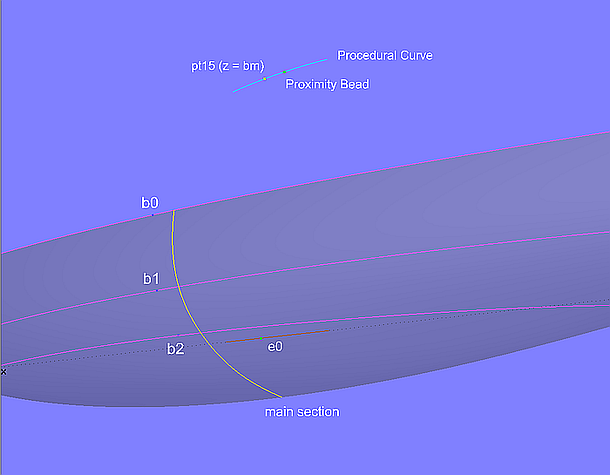
Model sk15-1.ms2 - determination of main section according to the square metre class rules
Model sk15-1.ms2 - 15 sqm yacht hull
Mathematical functions available in MultiSurf
| Name | Argument(s) | Result | Synopsis |
| ABS | 1, any units | Same units as argument | Absolute value |
| ACOS | 1: unitless | unitless | arc cosine (radians) |
| ACOSD | 1: unitless | unitless | arc cosine (degrees) |
| ALARM | 2: any units | Unitless | ALARM has 2 arguments ALARM(x,y). The alarm "goes off" (goes into error) if (1) it is set (x > 0) AND (2) y < 0. Using a formula or expression for y, you can build various warning limits into a model. |
| ANGLE | 3: point, point, point | Unitless (degree) | Angle of three points (angle at pt2 between the directions to pt1 and pt3) |
| ARCLEN | 3: curve, unitless, unitless | Length | Arc distance along curve, from t1 to t2 |
| AREA | 2: surface, use_sym (0 or 1) | Area = L^2 | Area of surface, CompSurf, or TriMesh |
| ASIN | 1: unitless | unitless | arc sine (radians) |
| ASIND | 1: unitless | unitless | arc sine (degrees) |
| ATN | 1, unitless | Radian (unitless) | Arc tangent |
| ATND | 1, unitless | Degree (unitless) | Arc tangent (in degrees) |
| ATN2 | 2, both with same units | Radian (unitless) | Arc tangent(y/x) |
| ATN2D | 2, both with same units | Degree (unitless) | Arc tangent(y/x) (in degrees) |
| BBOX | 1. Entity or Entity List 2. Real scale factor 3. Real sign 4. Index, 1 to 3 for X, Y, or Z component | Length | The BBOX function gets information about the bounding box of an entity, or a set of entities specified by an Entity List. A bounding box is the smallest rectangular solid, aligned with the global coordinate system, that encloses the selected entities. |
| BSPL | 1. KnotList, or *UNIFORM for uniformly spaced knots. 2. K, polynomial order (2 for linear, 3 for quad-ratic, 4 for cubic, etc.) 3. N, number of basis functions. 4. I, index indicating which basis function to evaluate (1 to N). 5. T, parameter (nominal range 0 to 1, but can be any real value) |
unitless | The BSPL function evaluates the so-called “B-spline basis functions”, which are the mathematical foundations of B-spline and NURBS curves and surfaces. Example: BSPL( *UNIFORM, 3, 5, 2, 0.40) returns 0.3200. In this case the knots are uniform (0, 0, 0, 1/3, 2/3, 1, 1, 1); the B-splines are quadratic (K = 3); there are N = 5 of them; I = 2 selects the second basis function; T is 0.40. Errors: 222. NURB has too few knots for its order and num-ber of control points. 223. NURB has too many knots for its order and number of control points. 234. Insufficient spacing between knots. 556. BSPL function: order less than 1. 557. BSPL function: number of basis functions less than 1. 558. BSPL function: index is out of range (1 to num-ber of basis functions). |
| CEIL | 1: any units | Same units as argument | CEIL(x) is the smallest integer that is greater than or equal to x. |
| CENTROID | 3: entity, use_sym (0 or 1), index (1-3, for X,Y,Z coordinate) | Length | Coordinates of centroid |
| CLEAR | 2: point, graphic entity | Length | Clearance |
| COS | 1, radian (unitless) | Unitless | Cosine |
| COSD | 1, degree (unitless) | Unitless | Cosine (of angle in degrees) |
| COSH | 1: unitless | unitless | hyperbolic cosine |
| CURV | 1/Length | Curvature of host curve or snake, at t location of bead/ring. If t is on a breakpoint, hi_side (0 or 1) controls whether curvature is measured below or above the break. kind: 0 is 3-D curvature of curve or snake; 1 is nor-mal curvature of snake; 2 is geodesic curvature of snake. |
|
| CURVINT | 3: curve, t, real | L times units of real | Integral of real times ds along curve. ds is the element of arc length along the curve. t is a Variable. real is a Formula descended from t. |
| DIST | 2: point, point | Length | Distance between points |
| ERROR | 1: entity | Unitless | Error code attached to entity (0 if no error). |
| EXP | 1, unitless | Unitless | Exponential |
| FLOOR | 1: any units | Same units as argument | FLOOR(x) is the greatest integer that is less than or equal to x. |
| FRAMEPOS | 3: point, frame, index (1-3, for x,y,z coordinate) | Length | Coordinates of point in frame |
| GRAPH | 2: graph, unitless | Unitless | Evaluation of graph |
| HYDRO | 6: sp.gr., Zcg, sink, trim, heel, index | various, depending on index | Fixed-position hydrostatics based on the visible contours. index is 1 to 29; selects one of 29 results, e.g. index = 6 for displacement volume; index = 15 for wetted surface. |
| IF | 3: any units | Same as units of selected argument | If arg1 >0, arg2; else arg3 |
| LOG | 1, unitless | Unitless | Natural logarithm |
| LOG10 | 1, unitless | Unitless | Base-10 logarithm |
| MASS | 3: entity, use_sym, index | M ML |
Mass, if use_sym is not 0, includes symmetry images. Index = 0 returns Mass. Index = 1, 2 or 3, the value returned is the mass moment with respect to X, Y or Z. This is the product of mass times the X, Y or Z coordinate of the centroid. Unit dimensions are ML. |
| MAX | 2, both with same any units | Same units as arguments | Maximum |
| MIN | 2, both with same any units | Same units as arguments | Minimum |
| PI | 1; any units | Unitless | PI has 1 argument, but its value is immaterial; PI(x) = pi for any x. |
| ROUND | 1, any units | Same units as argument | Rounding to integer |
| ROUND2 | 1, any units | Same units as argument | ( x, places) rounds x to the specified number of decimal places. E.g., ROUND2(PI(0),2) is 3.140000. |
| SIGN | 1: any units | Unitless | SIGN(x) is +1 when x > 0, -1 when x < 0, 0 when x = 0. |
| SIN | 1, radian (unitless) | Unitless | Sine |
| SIND | 1, degree (unitless) | Unitless | Sine (of angle in degrees) |
| SINH | 1: unitless | unitless | hyperbolic sine |
| SQRT | 1, unit dimensions all multiples of 2 | Unit dimensions of argument divided by 2 | Square root |
| STRAIN | 2: Surface/TriMesh, index | Unitless | Surface/TriMesh is a surface or TriMesh entity index = 0 or 1, for minimum or maximum strain This function reports the strain range for an Expanded Surface or Expanded TriMesh. |
| SURFCURV | 5: magnet, hi_side_u, hi_side_v, kind, angle | L^-1 for kind = 0 or 2; L^-2 for kind = 1 | Surface curvature kind = 0, normal curvature kind = 1, Gaussian curvature kind = 2, mean curvature |
| SURFINT | 4: surface, u, v, real | L^2 times units of real | Integral of real times dA over surface dA is the element of area on the surface u and v are Variables real is a Formula descended from u and v. |
| TAN | 1, radian (unitless) | Unitless | Tangent |
| TAND | 1, degree (unitless) | Unitless | Tangent (of angle in degrees) |
| TANH | 1: unitless | unitless | Hyperbolic tangent |
| TPOS | 1, bead or ring | Unitless | t parameter |
| UNITMASS | 1: entity | M for a point ML^-1 for a curve ML^-2 for a surface ML^-3 for a solid |
unit weight property of entity |
| UPOS | 1, magnet or ring | Unitless | u parameter |
| VELOCITY | 3: curve, t, hi_side | Length | Rate of change of arc length with respect to t If t is on a breakpoint, hi_side (0 or 1) controls whether velocity is measured below or above the break. |
| VOLUME | 2: solid, use_sym (0 or 1) | Volume = L^3 | Volume of solid |
| VPOS | 1, magnet or ring | Unitless | v parameter |
| XPOS | 1, point | Length | X coordinate |
| YPOS | 1, point | Length | Y coordinate |
| ZPOS | 1, point | Length | Z coordinate |
======================================================================================