B-spline Curves and B-spline Surfaces
Properties and Applications
by Reinhard Siegel
Content
Introduction
1 B-spline Curve
- 1.1 Basics
- What does a B-spline Curve look like?
- Polyline similarity
- Degree
- Tangential property
- Cp shift - local effect
- Curvature profile
- 1.2. Applications
- B-spline Curve as support curve for surfaces
- Tangential joint of bow mc and fairbody curve
- Radius Arc and B-spline Curve
2 B-spline Surface
- 2.1 Basics
- Degree
- Local control
- Tangential property
- 2.2 Applications
- Round bilge hull
- Hull surface including bowround
- Planar surface
- Tangent plane
3 B-spline Lofted Surface
- 3.1 Basics
- C-spline Lofted Surface vs. B-spline Lofted Surface
- 3.2 Applications
- Examples from tutorials 8, 10 and 13
- Particular geometry of hull bottom surface
- Hull with propeller tunnel
Introduction
B-spline Curves in MultiSurf are easy to shape with a few control points, they do not oscillate, they always start and end in the same way. These geometric properties turn them into very practical freeform curves, for example as master curves for hull, deck or superstructure. B-spline Surfaces as their extension also have these geometric features. The following sections will show how B-spline Curves and B-spline Surfaces can solve many geometry tasks.
Abbreviations used:
cp: control point (support point)
mc: master curve = support curve
cp1, cp2, ...: denotes 1st, 2nd, ... point in the list of supports of a curve. It is not an actual entity name.
mc1, mc2, ...: denotes 1st, 2nd, ... curve in the list of supports of a surface. It is not an actual entity name.
In the following the terms used for point, curve and surface types are those of MultiSurf. This may serve the understanding and traceability.
1 B-spline Curves
1.1 Basics
What does a B-spline Curve look like?
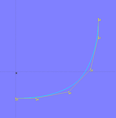
The parents of a B-spline Curve are a series of control points (cps). This can be free points in space (Points), or points on curves or surfaces (Beads, Rings, Magnets). The connection of the cps by straight lines is the polyline of the B-spline Curve. Model b-spline_curve-1.ms2 shows an example.
Model b-spline_curve-1.ms2 – relationship between arrangement of cps and curve form
Polyline similarity
The shape of the B-spline Curve is closely related to the shape of the polyline. The curve starts at the first cp and ends at the last cp, but does not pass through the inner cps, it imitates the polyline (approximation). This is in contrast to the C-spline Curve, which always passes through all control points (interpolation). One can think of the cps of the B-spline Curve as springs that tighten the curve.
Curve comparison – the B-spline Curve is "soft", closely following the polyline through its control points. A C-spline Curve behaves like a batten.
The B-spline Curve is "soft", it does not osscilate. The C-spline curve behaves like a fairing batten. A clearly bend curve can be modeled by a B-spline Curve with fewer control points than with a C-spline Curve.
The B-spline Curve is not determined from start to end by a single mathematical formula, but by several piecewise defined functions. Corresponding boundary conditions ensure that the transition from one section to the next is without gap, kink (steady slope) or curvature discontinuity (steady curvature).
Degree
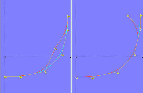
Apart from the arrangement of cps the parameter “Degree” of the B-spline Curve is important. This is evident from model b-spline_curve-2.ms2.
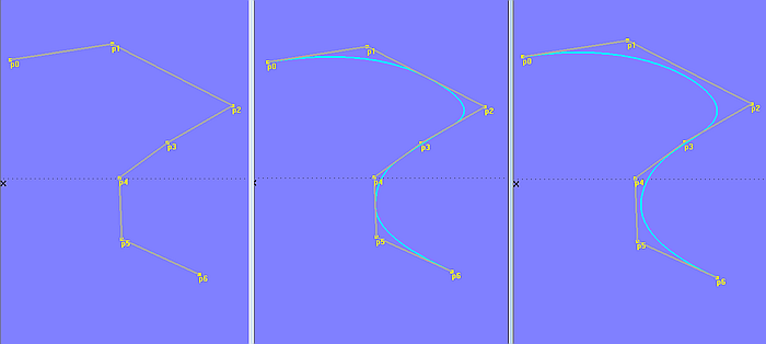
Model b-spline_curve-2.ms2 – the value of the parameter "Degree" determines how close the curve will follow its defining polyline (left: Degree = 1, center: Degree = 2, right: Degree = 3)
With Degree set to 1, the curve is identical to its polyline, it runs straight from point to point. When Degree is set to 2, the curve touches the midpoint of each inner segment of the polyline. At Degree = 3 the B-spline Curve is even more loosely guided. The higher the degree of the B-spline Curve, the “stiffer” the curve behaves, i.e. it more loosely imitates the polyline and has a higher number of continuous derivatives.
The maximum possible value for the degree of the B-spline Curve is n -1, where n is the number of its cps.
Tangential property
The above figures also reveal that the B-spline Curve always starts tangent to the first polyline segment, and always ends tangent to the last polyline segment. This tangential property is of very practical use.
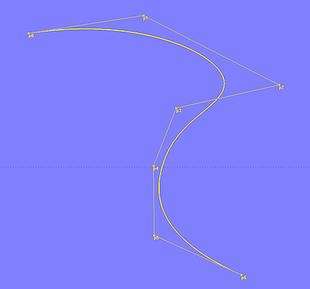
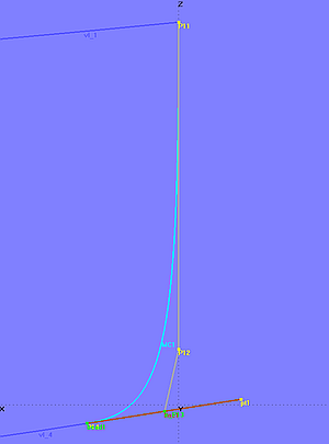
For example, if, as in model b-spline_curve-3.ms2, cp1 and cp2 of a master curve lie vertically one above the other (equal Y-coordinates), then the curve starts vertically (no flare, no tumble-home), no matter how cp3 is arranged. Should the mc end normal to the centerplane, the Z-coordinates of the last cp and the last but one cp must match.
By means of the tangential property of the B-spline Curve such geometric relationships can easily be hard-wired in the model.
Model b-spline_curve-3.ms2 – the tangential property of the B-spline Curve is of advantage. For example, to make a master curve start vertically and end horizontally.
Cp shift – local effect
B-spline Curves show another feature. When a cp of a B-spline Curve is moved, only a portion of it changes its shape. This is the result of the piecewise defined curve functions. For example, When the starting point of a B-spline Curve of degree-2 is moved, the shape changes only until to the middle of the polyline segment between the 2nd and 3rd cp, everything else remains the same. See model b-spline_curve-3a.ms2.
Model b-spline_curve-3a.ms2 and b-spline_curve-3b.ms2 – local influence of control points
When an inner control point is moved, the curve shape is modified only in its vicinity (model b-spline_curve-3b.ms2). Control points of the B-spline Curve have only a local effect on the run of the curve. The higher the value for degree, the more changes are effective to the entire form.
Curvature profile
A curve is fair if its curvature changes harmoniously along the curve. Via main menu/ View/ Display/ Profile/.Curvature or the corresponding toolbar button the curvature distribution can be displayed.
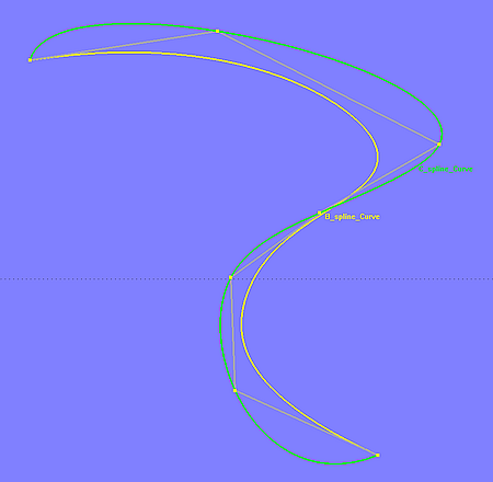
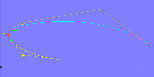
On the basis of model b-spline_curvature.ms2 the effect of the arrangement of the control points on the curvature profile is explained. Curve c0 (degree-3) shows in the region of maximum curvature a sudden drop – the curvature first decreases, then increases again, the distribution is inharmonious. In contrast, curve c1 (degree-3) shows a harmonic distribution of curvature. Both curves are superimposed, i.e. have the same shape, just the position of the inner cps is different.
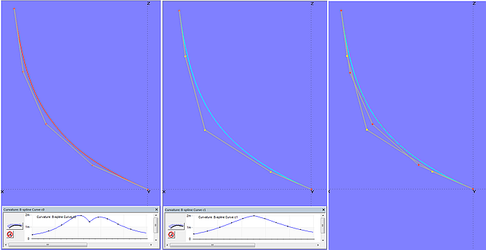
Model b-spline_curvature.ms2 – both B-spline Curves are superimposed, but their curvature profile is different.
That you can get with the same number of cps, but with a slightly different arrangement of the inner cps the same curve shape, is another special feature of B-spline Curves. A harmonic curvature distribution along the curve is preferable. Often it is sufficient to move the second and the second but last cp a little bit closer to the start and end of the curve to fix a local drop of curvature.
1.2 Applications
B-spline Curve as support curve for surfaces
The B-spline Curve is easy to shape with few control points (cps), it does not osscilate between its cps. Except for the first and the last cp it does not pass through its control points, but the shape of the curve always resembles the polyline through its cps. In addition, the B-spline Curve is always tangent to the polyline at its endpoints. This tangential property is very useful if a specific direction is wanted at the curve ends.
Hull surfaces
The hull of a boat or a yacht has more curvature in the transverse than in the longitudinal direction. With B-spline Curves one can create master curves for all kinds of main sections, from round bilge to long keel. For the same curve shape a C-spline Curve would require more control points, thus more efforts are needed for fairing.
Deck, superstructure, keel
Few control points, close imitation of its polyline and the tangential property - with these advantages B-spline Curves can also be used to model surfaces for decks, superstructures, keels, etc. Thereby they are suitable as supporting curves or as generating curves (B-splineLofted Surface).
Examples are presented in section 3.2.
Tangential joint of bow mc and fairbody curve
Model tangent_bow_mc.ms2 shows how to permanently join a B-spline bow master curve tangent to the fairbody curve of the hull.
Model tangent_bow_mc.ms2 – MC1 ends tangent to the fairbody curve, because e_P13 is a Bead on the tangent line at the start point of vl_4.
Radius Arc and B-spline Curve
A Radius Arc in combination with a B-spline Curve can be useful, for example, as a path for a Sweep Surface, the centerline of a pipe or for the outline of a window. Model RadiusArc_B-spline.ms2 shows the principle how both curves can be connected smoothly.
The Radius Arc of type-3 is tangent to line between point1-point2 and to line between point2-point3. A B-spline Curve is tangent to the end segments of its control polyline. So, in order to join a B-spline Curve tangent to a Radius Arc type 3 at its t=0 end, use a bead at t=0 on the Radius Arc as first cp and point1 as 2nd cp. This hard-wires tangency.
Model RadiusArc_B-spline.ms2 – smooth connection of B-spline Curve and Radius Arc
2 B-spline Surface
2.1 Basics
The control points of the B-spline Surface form a four-sided polygon net. Similar to the polyline of the B-spline Curve this net forms the surface. Except for the four corner points of the net, the control points are outside the surface. The shape of the B-spline Surface can be thought of as being connected to the interior control points by springs. The edges are all B-spline curves using control points from the four edges of the net. Model bsurf-1.ms2 shows an example.
Degree
Like the B-spline Curve, the B-spline Surface also has “Degree” parameters. There is a setting of degree in its longitudinal direction (u) and a setting of degree in its transverse direction (v).
The lower the values for degree, the closer is the surface to the polygon net. The higher the degrees, the “stiffer” the surface.
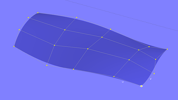
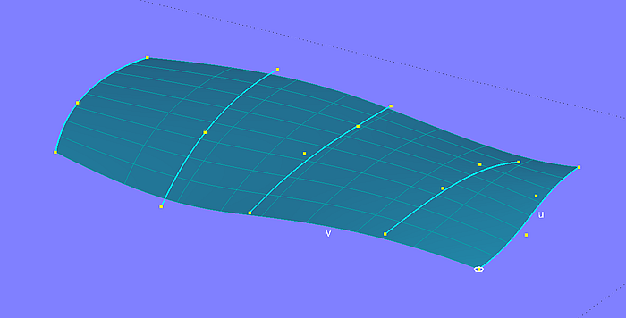
Model bsurf-1.ms2 – B-spline Surface with polygon net of control points (5 cps in u-direction, 4 cps in v-direction)
The B-spline Surface imitates its net of cps, it does not oscillate beyond. Except its corner points all cps lie outside the surface.
Local control
Similar to the B-spline curve, the effect of a control point on the shape of a B-spline Surface is local. See model bsurf-2.ms2. With increasing degree the influence of a control point becomes more global.
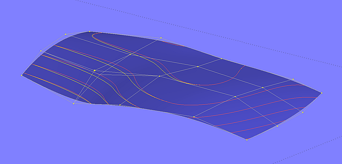
Model bsurf-2.ms2 – red and yellow sections illustrate the local effect of shifting a control point.
Tangential property
Similar to the B-spline Curve, the B-spline Surface also offers a tangency property. See model bsurf-3.ms2. This property can be used with advantage as shown in the following section about B-spline Surface applications.
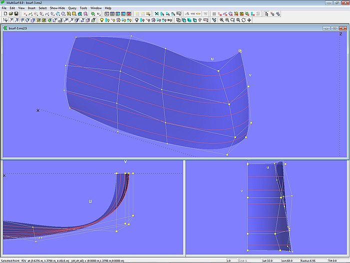
Model bsurf-3.ms2 – the cps in the v-direction of the 1st and 2nd column are perpendicular to each other. The B.spline Surface starts normal to the centerplane along the edge u = 0.
2.2 Applications
Round bilge hull
Model bsurf_hull.ms2 shows a round bilge hull defined by 5 x 4 control points.
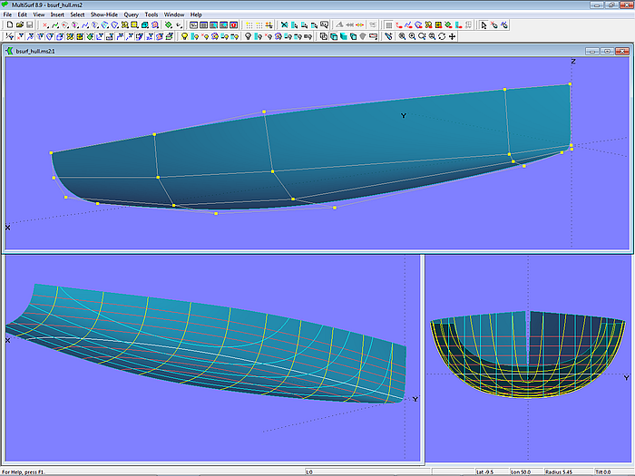
Model bsurf_hull.ms2 – B-spline Surface of a round bilge hull (5 x 4 cps)
The model uses the tangential property of the B-spline Surface in order to make the surface end normal to centerplane along the fairbody curve. All cps of this edge on centerplane (P24, P34, P44, etc.) have the same Z-coordinate as their corresponding neighbours (P23, P33, P43 etc.).
Hull surface including bowround
Model bsurf_hull_w_bowround.ms2 is another example of how a particular form feature can be firmly installed by the tangential property of the B-spline Surface. Here the bowround is part of the hull surface, it is not a separate surface. The polygon net uses 6 cps in u-direction (longitudinal). To ensure the start of the surface normal to the centerplane the cps along the stem are Projected Points of the cps of the next column in v-direction.
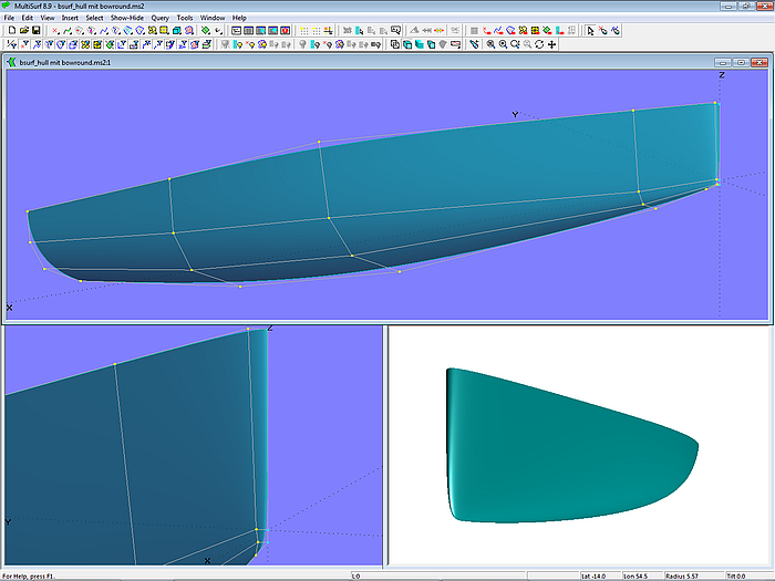
Model bsurf_hull_w_bowround.ms2 – the bowround is part of the hull surface.
Planar surface
Occasionally, a model requires a simple flat surface, for example, as a base surface for a frame or another planar component. A flat surface can also replace a 2-point Plane or 3-point Plane, which have the disadvantage to be displayed always as large as the entire model. This is detrimental with regard to clarity - what is needed only locally, does not need the extend of the whole model.
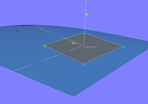
A planar surface can be created in different ways. For example by a Translation Surface, with Line entities each for generator and guiding curve. Or as a Ruled Surface spanned between two parallel Lines. With the minimum number of entities it can be created by a B-spline Surface at 2 x 2 cps. This is shown in model planar_bsurf.ms2. The 3 Points p1, p2 and p3 determine the position of the surface in 3D space, while the Copy Point p4 ensures that all 4 points lie in one plane. With these 4 points the B-spline Surface planar_surface is defined; degree in u- and v-direction is set to 1.
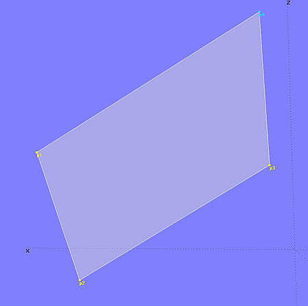
Model planar_bsurf.ms2 – flat surface with minimum of entities by B-spline Surface (degree = 1 in u- and v-direction)
Flat B-spline Surface as base for a hull frame
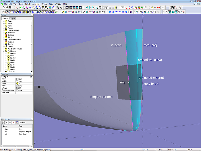
Tangent plane
In model tangent_bsurf.ms2 the construction of the tangent plane in a point on a surface is demonstrated. With Magnet m0, Offset Point pt01 and Point pt02 relative to m0 the 3-point Frame F0 is defined. In the YZ-plane of the frame Point p1 is positioned, a corner of the tangent plane. Point p1 is now mirrored against the Y-axis of the frame as Mirror Point p2 (2nd corner point), as well as against the Magnet m0 as Mirror Point p3 (3rd corner). The 4th corner is Copy Point p4. Finally, with these points the B-spline Surface tangent_surface is created.
Model tangent_bsurf.ms2 – B-spline Surface as tangent plane at Magnet m0
Moving m0 changes the whole construction accordingly. By p1 width and length of the flat surface can be adjusted according to the requirements.
Of course, a tangential plane at point m0 can also be created by a 2-point Plane entity with Magnet m0 and the Offset Point pt01. But in the way presented here, the size of the planar surface can be controled. In addition, its position in the model provides information about the purpose it serves. The model becomes more clear.
3 B-spline Lofted Surface
3.1 Basics
In a C-spline Lofted Surface the mcs are "planked" by C-spline Curves. If B-spline Curves are used instead, the result is a B-spline Lofted Surface.
Like the B-spline Curve which starts in the first cp and ends in the last cp, the B-spline Lofted Surface starts at the first mc and ends at the last mc. It does not interpolate the inner mcs, as a B-spline Curve does not run through its inner cps.
A B-spline Lofted Surface follows its mcs, it does not oscillate beyond it.
Curves of different types can be used as mcs of a B-spline Lofted Surface. For example, in the model bloftsurf.ms2 mc4 is a C-spline Curve, while mc5 is an Arc.
The B-spline tangential property is useful in many ways with the B-spline Lofted Surface. For example to connect the surface smoothly to another surface or make its edges start or end in a certain way.
Model bloftsurf.ms2 – B-spline Lofted Surface: master curves of different types are “planked” by B-spline Curves.
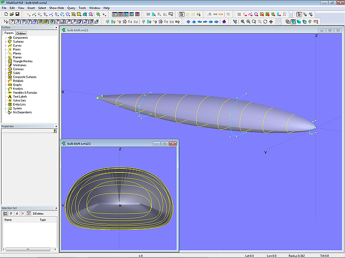
A B-spline Lofted Surface with all B-spline master curves of equal degree and equal number of cps is identical to a B-spline Surface with the same control points. However, because of its different organization the B-spline Lofted Surface is more manageable. The run of the mcs provides a clear impression of the shape of the surface in their vicinity.
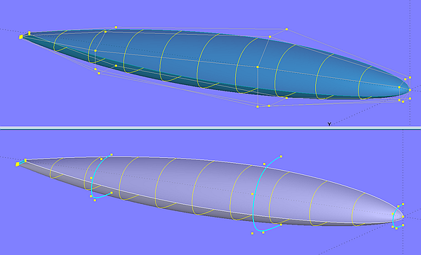
Models bulb_b-spline_surface.ms2 and bulb_b-spline_lofted_surface.ms2 – keel ballast bulb as B-spline Surface (top) and B-spline Lofted Surface (bottom)
C-spline Lofted Surface vs. B-spline Lofted Surface
A C-spline Curve is stiff, thus it needs more control points to bend it into a considerably curved shape. So a surface with intense curvature requires more mcs to create it by a C-spline Lofted Surface. B-spline Curves are soft, can be formed with a few cps and own the tangential property, what makes the B-spline Lofted Surface very attractive for surfaces with locally severe curvature.
3.2 Applications
Tutorials 8, 10 and 13 – B-spline Lofted Surfaces
The tutorials 8, 10 and 13 inform about application cases for B-spline Lofted Surfaces. Tutorial 8 (On the rounding of bows, sterns, sharp waterlines and on the attachment of keels) shows how bow and stern roundings can be created or how to connect a separate keel surface tangential to the hull. Tutorial 10 (On Keel Ballast Bulbs) and tutorial 13 (Decks and Superstructures) describe strategies and methods using B-spline Lofted Surfaces for ballast keels and superstructures.
Here are some examples. A detailed description can be found in the mentioned tutorials.
Attachment keel – hull
In model attached_keel.ms2 the keel of a classic sailing yacht including the tangential transition to the canoe body is defined by a B-spline Lofted Surface supported by 6 mcs. (Tutorial 8)
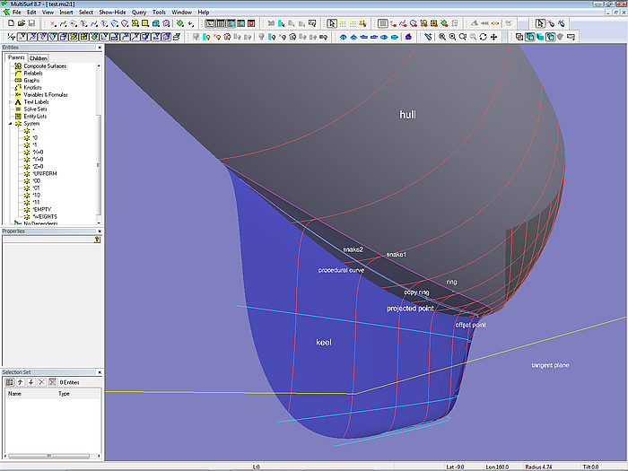
Model attached_keel.ms2 – keel (B-spline Lofted Surface) of a classic sailing yacht with tangential hull joint (Tutorial 8)
Bowround
Model tangent_bowround.ms2. (Tutorial 8)
Model tangent_bowround.ms2 – bowround by B-spline Lofted Surface (Tutorial 8)
Keel Ballast Bulb
The B-spline Lofted Surface offers full freedom in shaping bulbs for keel fins (model bulb_b-spline_lofted_surface.ms2). (Tutorial 10)
Model bulb_b-spline_lofted_surface.ms2 – ballast bulb by B-spline Lofted Surface; arrangement of master curves (Tutorial 10)
Superstructure
Model bubble_cabin_bloft-1.ms2 – round and soft transition between front, side and roof by B-spline Lofted Surface with transverse mcs. (Tutorial 13)
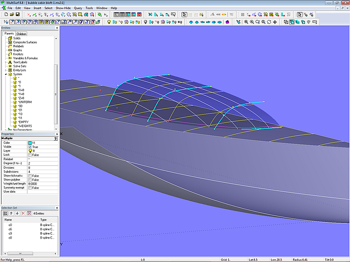
Model bubble_cabin bloft-1.ms2 – arrangement of master curves (Tutorial 13)
Here are two more examples which show the usefulness of the B-spline Lofted Surface.
Particular geometry of hull bottom surface
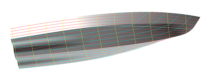
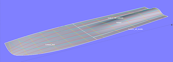
Model bottom.ms2 holds the bottom surface of a powerboat hull. It is a design requirement that aft of a fixed longitudinal position the buttocks run exactly straight.
For this purpose, the bottom surface is divided into two parts. Base of the aftbody is Translation Surface bottom_aft_0, created by Line l0 running in longitudinal direction and B-spline Curve mc_bottom_aft_0, which runs transversely. The forebody is defined by the B-spline Lofted Surface bottom_fwd, supported by 5 mcs. The forward 3 mcs are free B-spline Curves, but mc4 and mc5 are B-spline Snakes on the rear surface (bottom_aft_0). As a result, the forebody ends tangent on bottom_aft_0.
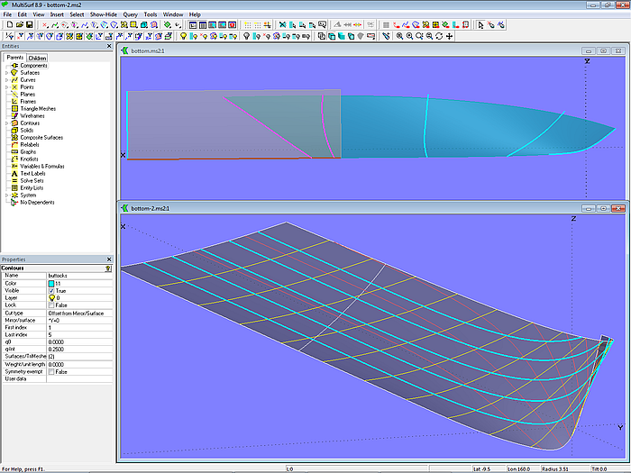
Model bottom.ms2 – bottom surface with straight buttocks in the aftbody
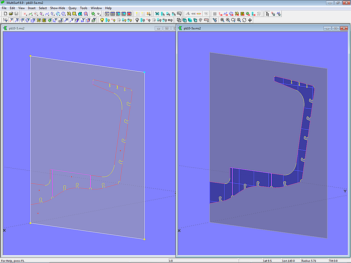
Hull with propeller tunnel
Model tunnel_stern.ms2 demonstrates how a propeller tunnel can be added to the bottom surface of a powerboat hull. Base of the bottom is C-spline Lofted Surface bottom_0. The tunnel surface is B-spline Lofted Surface tunnel, determined by 6 mcs running lengthwise.
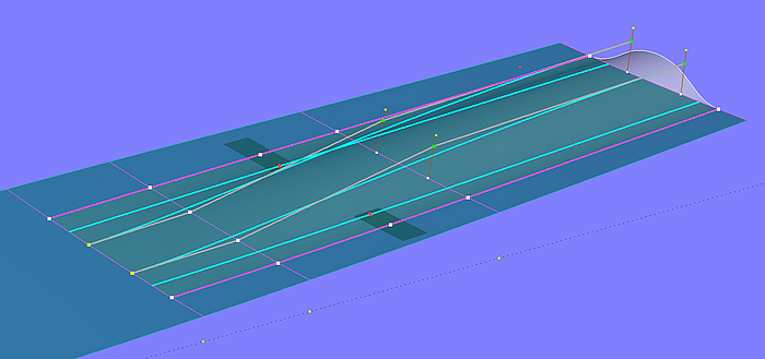
Model tunnel_stern.ms2 – propeller tunnel by B-spline Lofted Surface (6 mcs)
The edge mcs are B-spline Snakes on the bottom surface. The two mcs in the middle are B-spline Curves, shaping size and run of the tunnel top in transverse and longitudinal direction. The tangent attachment of the tunnel surface to the bottom base surface is hard-wired by the two Procedural Curves mc2_tunnel and mc5_tunnel. Their construction ensures that each curve point of these two mcs lies on the tangent plane of the corresponding curve point on the respective adjacent edge mc.
The final surfaces of the bottom are created by SubSurfaces.
Model tunnel_stern.ms2 –final bottom created by SubSurfaces
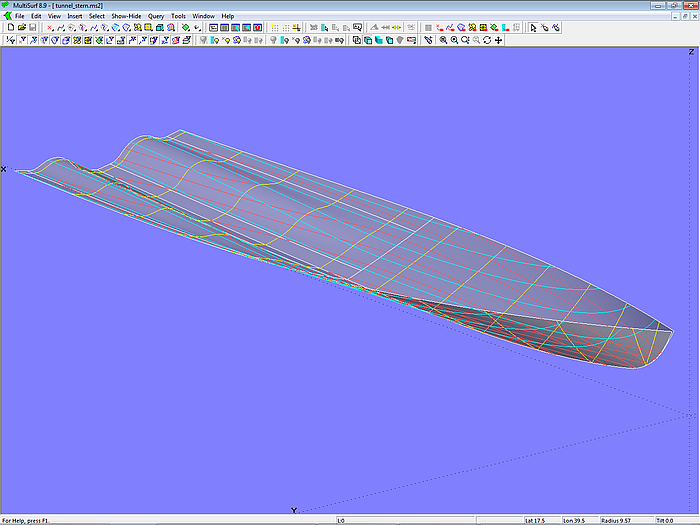
Model tunnel_stern.ms2 – powerboat bottom with propeller tunnel
======================================================================================