Form Features
About particularities of geometry of hull, deck and keel
by Reinhard Siegel
July 2020
Content
Introduction
1 Hull
- 1.1 - Full length chine - sailboat
- 1.2 - Vanishing chine - sailboat
- 1.3 - Vanishing chine – dinghy
- 1.4 - Vanishing chine - powerboat
- 1.5 - Hull bottom with straight buttocks
- 1.6 - Hull bottom with propeller tunnel
- 1.7 – Sprayrail
- 1.8 - Vanishing spraychine
- 1.9 - Washrail
2 Roundings
- 2.1 - Bow rounding
- 2.2 - Deck rounding 1
- 2.3 - Deck rounding 2
- 2.4 - Rounding of cabin edges
- 2.5 - Fin keel tip rounding
- 2.5 - Round transition between keel fin and ballast bulb
Introduction
Form features are special properties of geometry that, from the designer's perspective, are necessary for the functioning of his design. For example, a full length chine in the hull surface, a tunnel in the bottom, a characteristic hull-deck rounding. In the following, methods are described of how frequently required shape properties of hull, deck and keel can be modeled. Some designs have been covered in previous tutorials. However, they are listed here to create a comprehensive collection.
Abbreviations used:
cp: control point (support point)
mc: master curve = support curve
cp1, cp2, ...: denotes 1st, 2nd, ... point in the list of supports of a curve. It is not an actual entity name.
mc1, mc2, ...: denotes 1st, 2nd, ... curve in the list of supports of a surface. It is not an actual entity name.
In the following the terms used for point, curve and surface types are those of MultiSurf. This may serve the understanding and traceability.
1 Hull
1.1 Full length chine – sailboat
How to create a sailboat hull with a longitudinal chine is described in tutorial 2 "Round Bilge Hull With Full Length Chine". The hull in model sy15_full_length_chine.ms2 consists of two surfaces with a common longitudinal edge. For the topside a Developable Surface is used, the bottom is a C-spline Lofted Surface analogous to a standard round bilge hull. Along the longitudinal edge, the surfaces form a break in transverse direction that becomes weaker towards the bow.
Model sy15_full_length_chine.ms2 – a Developable Surface makes the topside, the bottom is a C-spline Lofted Surface with 6 master curves and 4 control points each (Tutorial 2).
1.2 Vanishing chine – saiboat
The modeling of a sailboat hull with a partial length longitudinal chine is the topic of tutorial 3 “Round Bilge Hull With Vanishing Chine”.
Model sy15_vanish_chine2.ms2 – vanishing chine. The rear mcs for side and bottom meet in transverse direction with a break, the front mcs adjoin each other tangentially (Tutorial 3).
The hull in model sy15_vanish_chine2.ms2 also consists of one surface for the topside and one surface for the bottom. Both are created like a standard round bilge hull. To ensure that the longitudinal chine gradually runs out, the rear mcs join with a transeverse break, while the front mcs connect tangentially.
Model sy15_vanish_chine2.ms2 – vanishing longitudinal chine (Tutorial 3
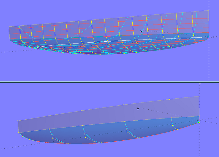
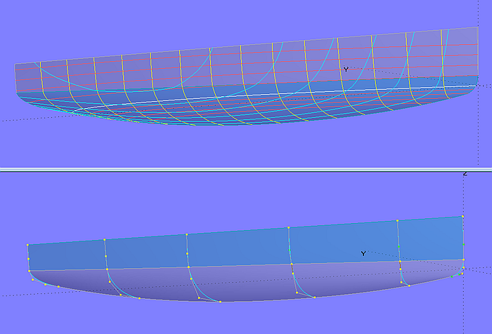
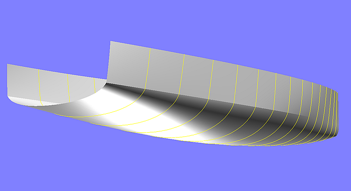
1.3 Vanishing chine – dinghy
In the two preceding modeling tasks, the hull consists of two partial surfaces which adjoin one another along the longitudinal chine or its extension. In model dinghy.ms2 the hull is one single C-spline Lofted Surface. The master curves run from the sheer of the hull to the bottom contour.
Model dinghy.ms2 – vanishing chine. Master curves running from sheer to bottom contour support a single C-spline Lofted Surface.
Except for the bow area, the master curves are PolyCurves; their components (B-spline Curves) adjoin with a break.
1.4 Vanishing chine – powerboat
If in the foreship area of a powerboat hull the stations should show considerable flare, a vanishing chine can prevent the deck from becoming excessively wide. Model powerboat_vanish_chine.ms2 is an application of the method described above (one single surface with chine). Mc2 and mc3 are PolyCurves; their components each are a Line and a B-spline Curve entity, joining with a break. All other mcs of the C-spline Lofted Surface are B-spline Curves.
Model powerboat_vanish_chine.ms2 – C-spline lofted Surface with partial length chine. Mc2 and mc3 are PolyCurves.
Model powerboat_vanish_chine.ms2
1.5 Hull bottom with straight buttocks
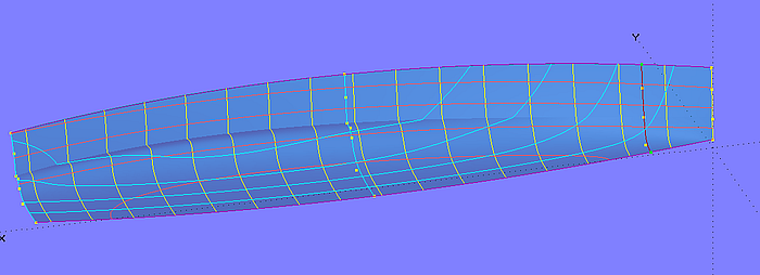
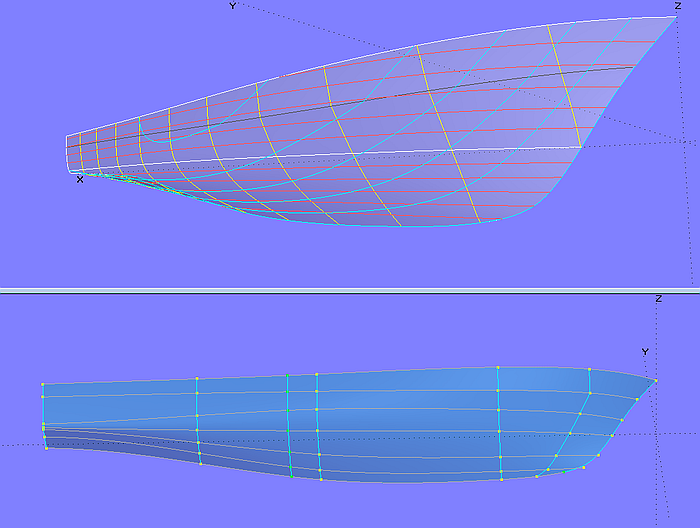
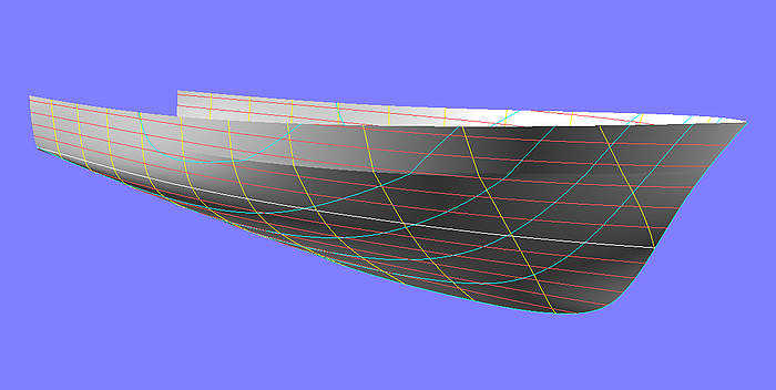
In tutorial 17 "B-spline Curves and B-spline Surfaces" the construction of a specially shaped bottom surface of a powerboat hull is described (model bottom.ms2). The design requirement is that aft of a fixed longitudinal position the buttocks run exactly straight.
For this purpose, the bottom is divided into a front part and a rear part. The base surface of the straight aft part is a Translation Surface, spanned between a Line in longitudinal direction and a B-spline Curve in transverse direction, which determines the cross section shape. The front part of the bottom is formed by a B-spline Lofted Surface, supported by 5 mcs. The forward 3 mcs are free B-spline Curves, but the last two mcs are B-spline Snakes on the Translation Surface. As a result, the forebody runs tangentially into the aftbody.
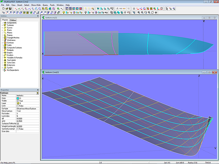
Model bottom.ms2 – bottom surface with straight buttocks in the aftbody (Tutorial 17)
1.6 Hull bottom with propeller tunnel
Also in tutorial 17 "B-spline Curves and B-spline Surfaces" the model tunnel_stern.ms2 shows how a propeller tunnel can be inserted into the bottom surface of a powerboat hull. The base surface of the bottom is a C-spline Lofted Surface, the tunnel surface is a B-spline Lofted Surface supported by 6 mcs running in longitudinal direction.
Model tunnel_stern.ms2 – propeller tunnel by B-spline Lofted Surface on 6 mcs (Tutorial 17)
The edge mcs are B-spline Snakes on the bottom surface. The two mcs in the middle are B-spline Curves, shaping size and run of the tunnel top in transverse and longitudinal direction. The tangent attachment of the tunnel surface to the bottom base surface is hard-wired by two Procedural Curves. Their construction ensures that each curve point of these two mcs lies on the tangent plane of the corresponding curve point on the respective adjacent edge mc.
The final surfaces of the bottom are created by SubSurfaces.
Model tunnel_stern.ms2 – final bottom created by SubSurfaces (Tutorial 17)
1.7 Sprayrail
Model sprayrail-1.ms2
Model sprayrail-1.ms2 shows how, with little effort, a sprayrail can be created that should run with a constant width from a certain point.
For the construction of a sprayrail the entity Relative Curve can be used conveniently. The parents of a Relative Curve are a base curve and two points. The start and end points of the base curve are moved to these points, and all intermediate points of the base curve are interpolated. A graph can be used to influence the interpolation of these intermediate points, for example to weight the rear point more than the front point.
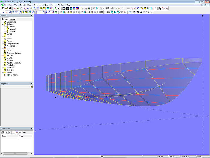
Model sprayrail-1.ms2 – construction of a sprayrail with Relative Curve
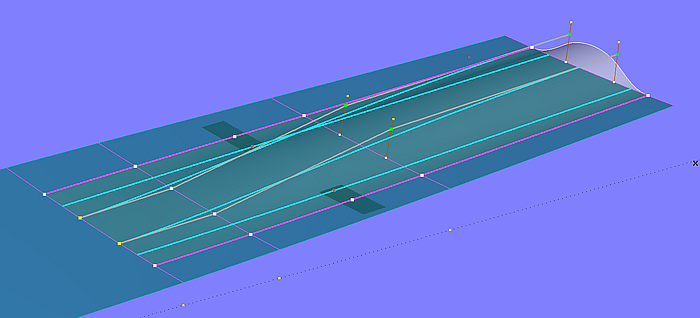
In model sprayrail-1.ms2 the starting point for the inside edge of the sprayrail is B-spline Curve sp_c0. It lies in the XY-plane and is projected onto the bottom of the hull as Projected Snake sp_n0. The Ring ring1 is located at the start point (t = 0) of sp_n0, the Ring ring2 at the end point (t = 1). The width of the sprayrail is determined by Point p1, which is offset in the Y-direction to ring2.
The outer edge of the bottom surface of the sprayrail is formed by the Relative Curve sp_c1. Its parents are as curve the snake sp_n0, as Point1 the Ring ring1, as Point2 the Point p1 and the B-spline Graph h1.
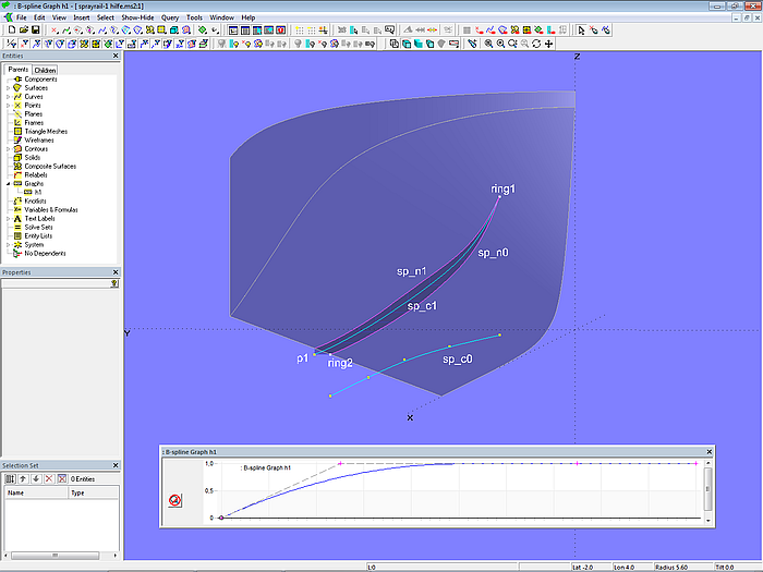
Model sprayrail-1.ms2 – the run of a Relative Curve can be modified with a B-spline Graph.
The B-spline Graph h1 has 4 values, the initial value is zero, the other values are equal to 1. This means that the point ring1 only plays a role at the beginning of the Relative Curve, then from a certain distance on only the Point p1 is taken into account in the interpolation. The shape of the B-spline Graph can be displayed using the function View/ Display/ Profile/ Graph.
For the side face of the sprayrail the Relative Curve sp_c1 is projected onto the hull bottom perpendicular to the XY-plane (Projected Snake sp_n1). Finally, with the 3 master curves sp_n1, sp_c1 and sp_n0 the B-spline Lofted Surface sprayrail is created.
The advantage of this construction is simplicity. But one has to experiment a little with the number of values equal to 1 for the B-spline Graph h1 in order to define the region with constant width of the sprayrail.
Model sprayrail-2.ms2
The PolyGraph entity is available in exactly the same way as the entity PolyCurve. It consists of several B-spline Graphs. In model sprayrail-2.ms2 the B-spline Graph h1 controls the increase of the sprayrail from zero width to maximum. The B-spline Graph h2 ensures that the width remains constant. The PolyGraph h3 binds the two graphs together. It is not necessary to adjust increase and constant width by a single graph, which makes the matter clearer. The PolyGraph also has the advantage that its end t values can be used to determine the distance over which the individual graphs are determinative. In the example model, the B-spline Graph h2 takes over from t = 0.25, so from 25% of the base curve the Relative Curve is parallel to it and thus the width of the sprayrail is constant.
Model sprayrail-3.ms2
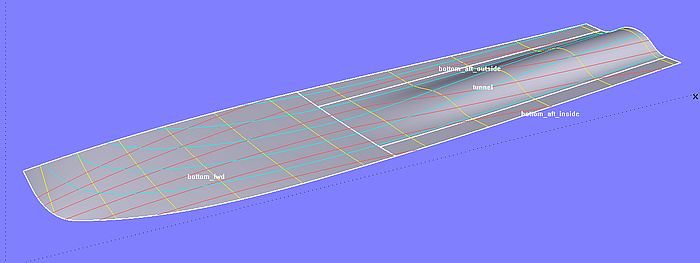
Model sprayrail-3.ms2 shows an example of how to model a sprayrail that starts with a less pointed front part, reaches a maximum width after a certain distance, and then remains constant up to the rear.
Starting point for the inside edge of the sprayrail is the B-spline Curve sp_c0 in the XY-plane. It is projected onto the hull bottom as Projected Snake sp_n0. The Ring ring1 is located at the start (t = 0) of sp_n0, Ring ring3 at the end (t = 1). Ring ring2 determines the length of the front part of the sprayrail, the joining main part between ring2 and ring3 is defined by the SubSnake sp_n1. This snake is the base curve for the Relative Curve sp_c1. With their dy- and dz-coordinate values, the two Points p1 and p2 (relative to ring2 and ring3) define the start and end widths as well as the lateral inclination of the main part of the sprayrail.
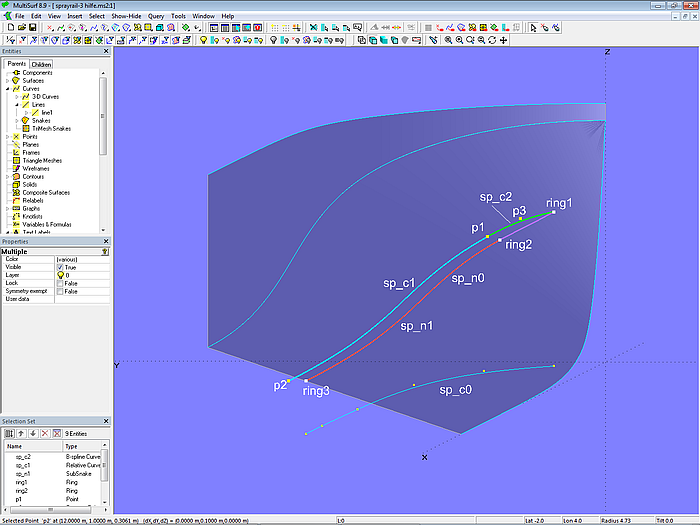
Model sprayrail-3.ms2 – sprayrail with blunt front part
The B-spline Curve sp_c2 shapes the increase in width in the front part. The Tangent Point p3 hard-wires, that sp_c2 connects to the Relative Curve sp_c1 smoothly. Both curves are combined into PolyCurve sp_c3, which in turn is then projected vertically onto the bottom as Projected Snake sp_n2.
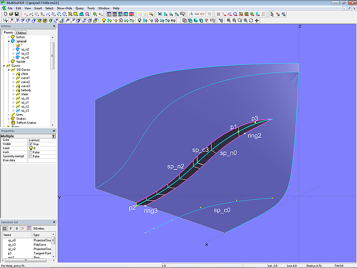
Model sprayrail-3.ms2 – sprayrail with blunt front part
The B-spline Lofted Surface sprayrail is created finally by the 3 master curves sp_n0, sp_c3 and sp_n2.
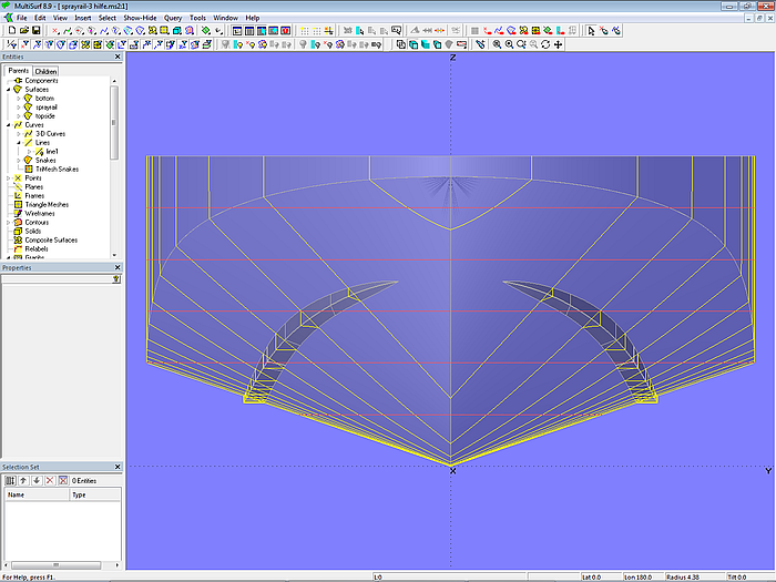
Model sprayrail-3.ms2 – sprayrail with blunt front part
1.8 Vanishing spraychine
In tutorial 12 “Vanishing Spraychine”, various methods are reported on how to model a spraychine that only extends over a part of the hull surface.
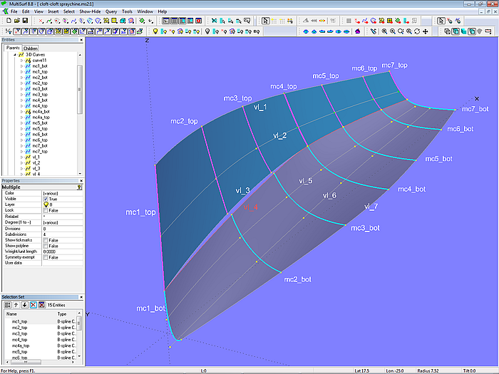
Model cloft-cloft-spraychine.ms2 – arrangement of master curves and guiding curves for fairing of the C-spline Lofted Surfaces topside and bottom (Tutorial 12)
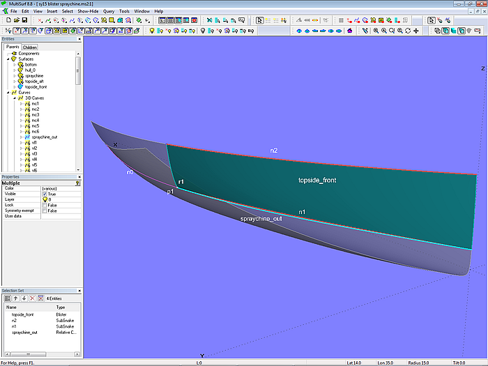
Model blister-spraychine.ms2 – Blister surface topside_front (Tutorial 12)
1.9 Washrail
Model washrail.ms2 demonstrates how a toerail or washrail can be modeled for a metal boat hull. The design requirements for the washrail are a constant width of its top face, and the inside face should be perpendicular to the deck.
The C-spline Lofted Surface hull_0 (5 mcs with 5 cps each) is the starting point. The deck surface deck_0 is also a C-spline Lofted Surface with the same number of master curves. With every deck-mc, the first cp lies as XYZBead on the corresponding hull-mc, namely by the height of the washrail below the first cp of the hull-mc. This arrangement has the advantage that one can see the final freeboard when modeling the hull.
The extent to which the first cp of the deck-mcs is below the upper edge of the hull is determined by the Variable washrail_height. So the height of the washrail can quickly be changed. On the other hand, the height remains the same if the sheerline of the hull is changed.
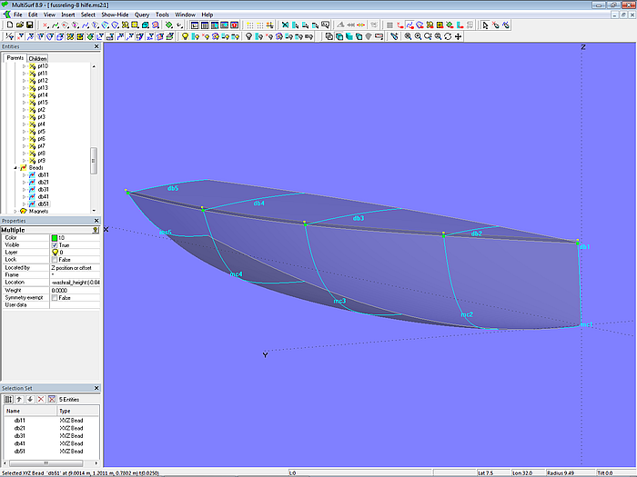
Model washrail.ms2 – the outer edge of the deck is below the sheer of the hull by the height of the washrail. The first cp of each deck-mc is a bead on the corresponding hull-mc.
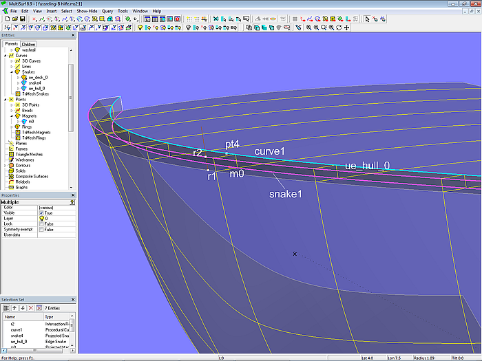
First the EdgeSnake oe_deck_0 is created along the outer edge of the base surface of the deck (C-spline Lofted Surface deck_0). It is support for Ring r1, on which the Tangent Point pt1 and the Offset Point pt2 depend. Line l0 connects r1 and pt2. Now pt1 is rotated by 90° around this line (Rotated Point pt3), which is then projected onto the deck as Projected Magnet m0.
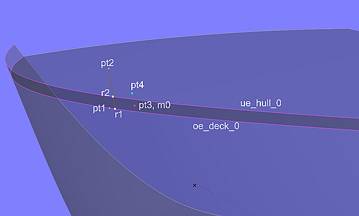
Model washrail.ms2 – definition of a curve point for the procedural construction of the inner edge of the washrail
At the position of Ring r1, the upper edge of the hull (EdgeSnake ue_hull_0) is then cut in XYZRing r2. With the three points r1, m0 and r2 generated in this way, the point pt4 is defined as Copy Point.
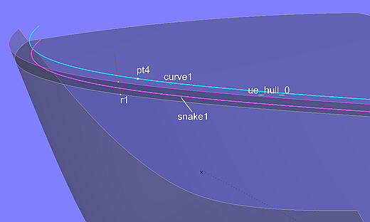
Model washrail.ms2 – construction of the inner edge of the washrail as a Procedural Curve
This construction of the point pt4 is now repeated for all positions of Ring r1 by the Procedural Curve curve1. Its perpendicular projection onto the deck is snake1.
Finally the surface washrail is created as a B-spline Lofted Surface with the three longitudinal curve supports ue_hull_0, curve1 and snake1.
Model washrail.ms2
2 Roundings
2.1 Bow rounding
In tutorial 8 “On the rounding of bows, sterns, sharp waterlines and on the attachment of keels” different constructions for bow rounding are presented. The method preferred by the author will now be shown by means of the model tangent_bowround-2.ms2.
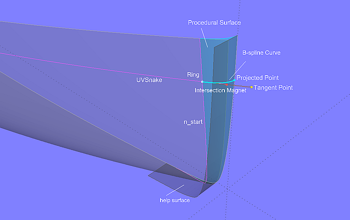
Model tangent_bowround-2.ms2 – tangential bow rounding by Procedural Surface
The Ring ring1 is located on the snake n_start, which determines the beginning of the bow rounding, as a support for a longitudinal UVSnake. The tangent at the position of ring1 is then created with the help of Tangent Point pt3 on this snake. The Line from ring1 to pt3 intersects the stem help surface (perpendicular to the midship plane) in the Intersection Magnet m3. This Intersection Magnet is then projected onto the midship plane as Projected Point pt4. The points ring1, m3 and pt4 are now the parents of the B-spline Curve curve1. Finally, the construction of this curve is repeated by a Procedural Surface for all positions of ring1. That is, the moving curve of the Procedural Surface is curve1, the driving point is ring1.
Note:
It is important that the tangent intersects the help surface (Intersection Magnet m3). If the help surface intersects the tangent in an Intersection Bead and this one is used as parent for pt4 and curve1, the calculation of the bow rounding takes more time.
2.2 Deck rounding 1
Rolling Ball Fillet
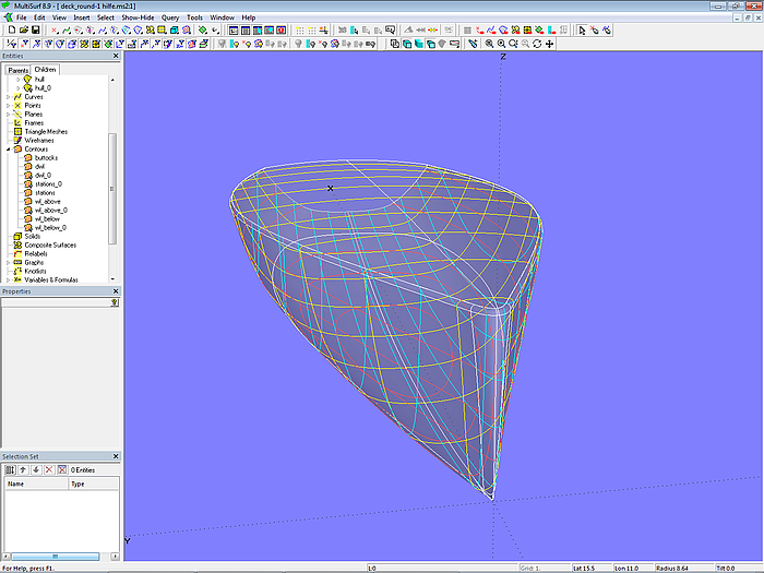
Model deck_round-1.ms2 demonstrates how the edge between deck and hull can be rounded off using surfaces of the type Rolling Ball Fillet.
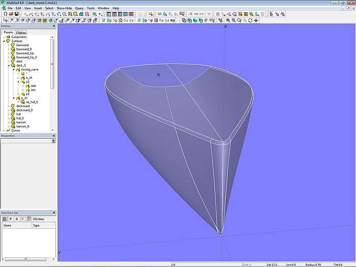
Modell deck_round-1.ms2 – rounding between hull and deck with Rolling Ball Fillets
The starting point are the base surfaces hull_0 and deck_0, which join together along the upper edge of the hull, as well as the bow rounding bowround_0. The rounding between hull and deck is done by the Rolling Ball Fillet deckround_0, the rounding between bow and deck by the Rolling Ball Fillet bowround_top_0. The Variable radius defines the size of both roundings.
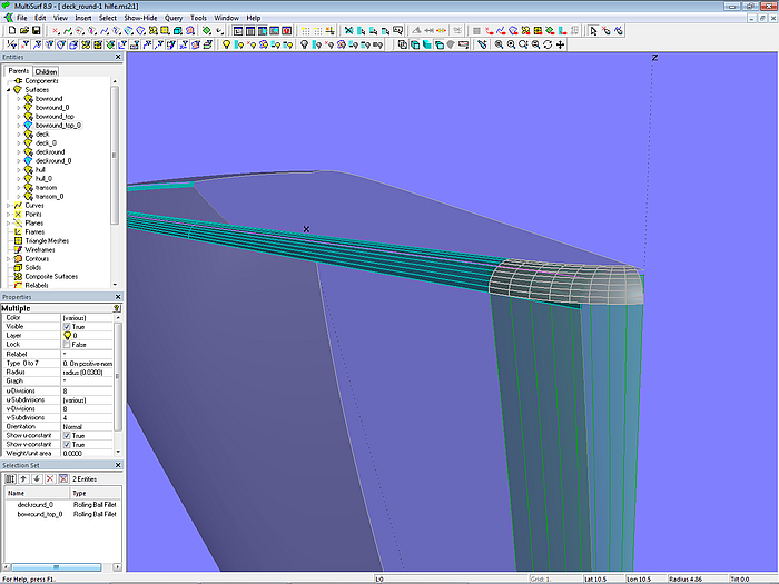
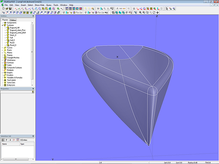
Modell deck_round-1.ms2 – rounding between hull and deck with Rolling Ball Fillets
To get their uncovered parts, hull, deck and bow are finally cut off on the rounding surfaces (SubSurface hull, Trimmed Surface deck, Trimmed Surface bowround).
Modell deck_round-1.ms2 – rounding between hull and deck with Rolling Ball Fillets
2.3 Deck rounding 2
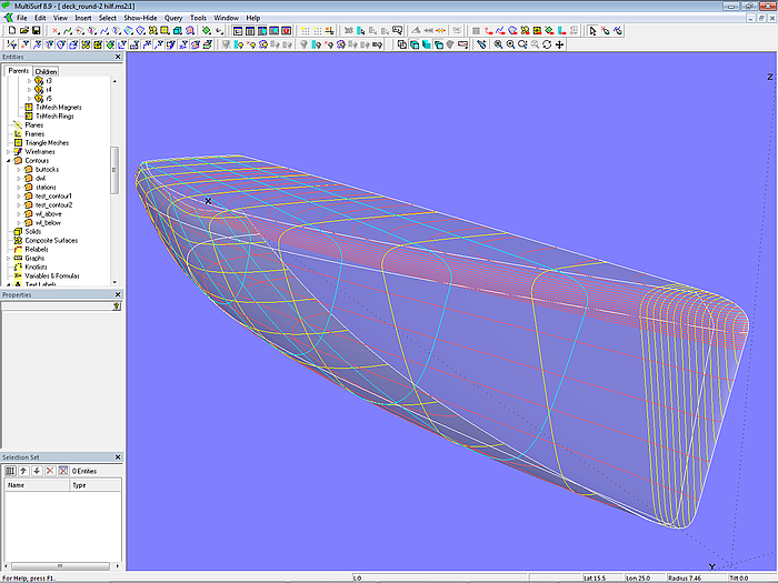
While in model deck_round-1.ms2 the rounding between hull and deck shows a relatively small radius which is constant over the length, the rounding in model deck_round-2.ms2 is a free-form surface.
Model deck_round-2.ms2 – large hull-deck rounding
The base surfaces of hull and deck (hull_0; deck) are C-spline Lofted Surfaces with 5 B-spline master curves each. This type of surface is also used for the base surface of the rounding between hull and deck (deckround_0).
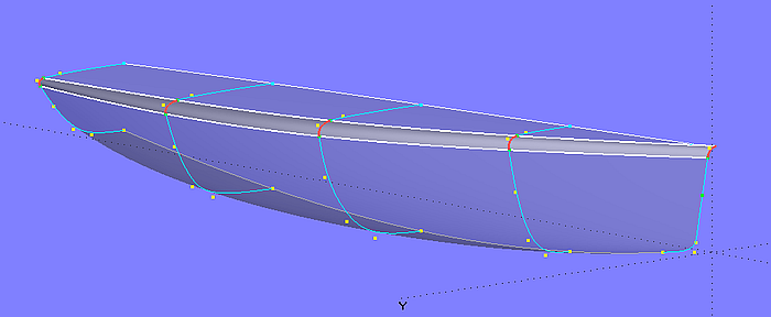
Model deck_round-2.ms2 – base surfaces of hull, deck and rounding as C-spline Lofted Surfaces
The mcs of the hull-deck rounding are defined by 3 cps each. Cp1 is a bead on the line connecting the first cp of the hull-mc and the second cp of the deck-mc. And cp3 is a bead on the line connecting the first and second cps of the hull-mc. In this way the tangential joint of the rounding mc is established to both hull and deck mc.
Let us take mastercurve 3 as an example. The B-spline Curve mc3_round is defined with the Bead e31, the Point p31 and the Bead e32. e31 lies on Line l_31, which connects Point p31 and p32 (cp1 and cp2 of the hull-mc). The Bead e32 is on Line l_32 between Point p31 and Point d32, the cp2 of the deck-mc.
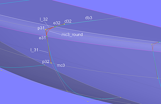
Model deck_round-2.ms2 – tangential joining of the rounding mc with the mcs of hull and deck
The bow is rounded in standard fashion by the B-spline Lofted Surface bowround. Control curves (parents) are snake n0 on the hull, defining the beginning of the rounding, the first control curve of the hull mc1 and its projection onto the midship plane, Projected Curve c0.
The rounding bowround_top, which creates the transition between bow rounding (bowround), deck (deck) and hull-deck rounding (deckround_0), is a Tangent Boundary Surface. Its definition requires 4 curves. Curve1 is the EdgeSnake le_deck along the front edge of the deck (deck), curve2 is the B-spline Curve c1 on the midship plane, which runs tangentially to both deck and bow centerlines with the help of 2 Tangent Points. Curve3 is the EdgeSnake ue_bowround, the upper edge of the bow rounding surface bowround. Curve4 is the B-spline Snake n2, which defines the entry of bowround_top into the hull-deck rounding deckround_0. By specifying appropriate boundary conditions, the Tangent Boundary Surface bowround_top runs tangentially to the bow rounding, to the hull-deck rounding and to the deck as well as normal to the midship plane.
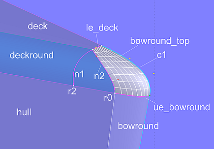
Model deck_round-2.ms2 – the Tangent Boundary Surface bowround_top is tangential to the adjacent surfaces and normal to the midships plane.
Model deck_round-2.ms2
2.4 Rounding of cabin edges
With the surface type Rolling Ball Fillet, the edges along the roof of a deck cabin can also be rounded off. Tutorial 13 “Decks and Superstructures” shows examples.
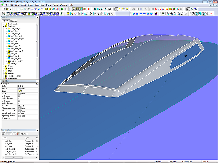
Model trunk_cabin_round_edges.ms2 – rounding the edges of a deck cabin with Rolling Ball Fillets (Tutorial 13)
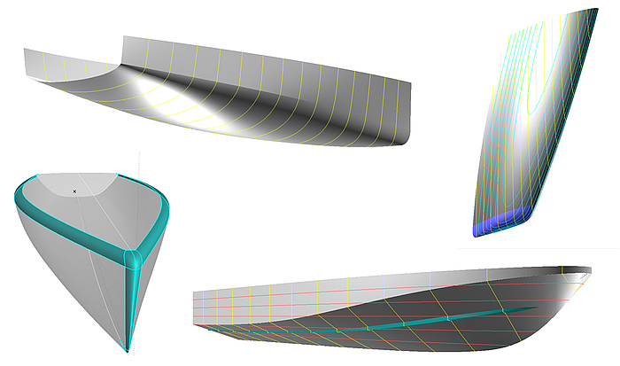
2.5 Fin keel tip rounding
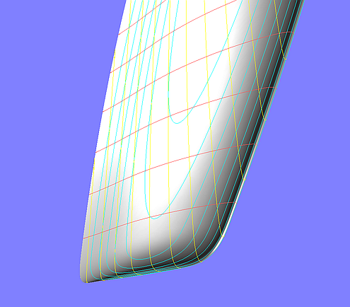
The tip edge of a keel fin should be rounded off. Model fin_keel_tipround.ms2 shows how a Blend Surface can be used for this task. A Blend Surface creates a smooth transition between two surfaces.
The base of the fin keel is the C-spline Lofted Surface fin_keel_0, which interpolates 3 master curves of the curve type Foil Curve.
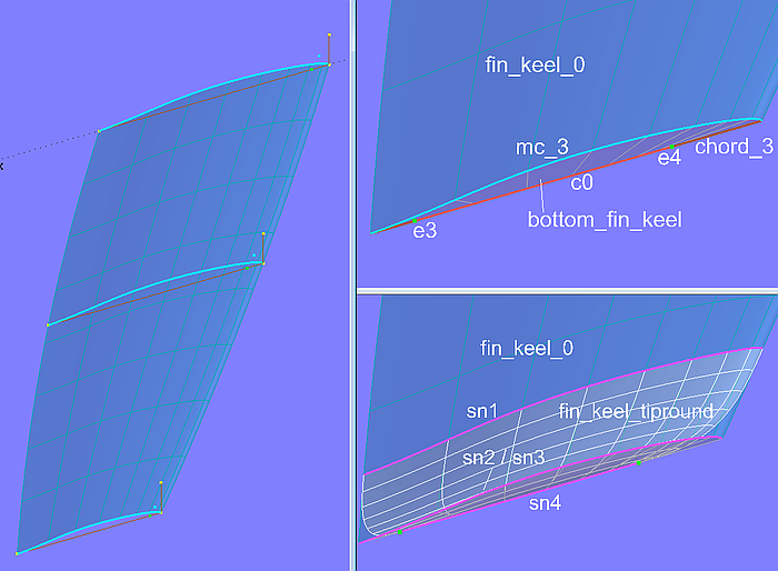
Model fin_keel_tipround.ms2 – keel tip rounding with Blend Surface
The flat keel sole is the Ruled Surface bottom_fin_keel, spanned between the lower keel mc mc_3 and the SubCurve c0. Its two defining Beads e3 and e4 are located on the tip section chord chord_3.
A Blend Surface requires 4 supports: two snakes on surface 1 and two snakes on surface 2. The start of the Blend Surface fin_keel_tipround is determined by Snake sn1. In the example here, this is a simple Line Snake between a Ring on the keel trailing edge and a Ring on the keel leading edge. The EdgeSnake sn2 runs along the tip edge of the keel fin. Along the outer edge of the keel sole surface bottom_fin_keel the EdgeSnake sn3 takes its course, along its inner edge the EdgeSnake sn4. So the required snakes for the rounding of the two surfaces are determined.
The rounding in the corners can be modified by the two Beads e3 and e4. To just round off the keel outline at the front, move e3 to the rear end of the tip chord chord_3.
Note:
SubCurve c0 is defined with the Relabel entity label.
Why?
Curve velocity is the rate of change in distance (arc length) along the curve in relation to the change in the t parameter value. For example, without a relabel, the speed of a line or an arc is constant – the same t-intervals have exactly the same arc lengths. With a B-spline Curve however, the speed depends on the distance between the control points. It is low in regions where two or more control points are close together, and relatively high when the control points are far apart. For most types of curves, curve velocity is variable with respect to t.
The velocity distribution along a curve can be visualized by displaying the tickmarks (Properties Manager). If tickmarks are close together, the speed is low, if they are further apart, it is high. Alternatively, one can also display curve velocity via View/ Display/ Profile/ Velocity Profile.
The master curves of the keel fin fin_keel_0 are Foil Curves. Their curve velocity in relation to t is zero at the leading edge (t = 1). This is passed on to all dependent snakes. Therefore three of the snakes defining the Blend Surface (Line Snake sn1 and Edge Snakes sn2 and sn3) also have a curve velocity of zero at the leading edge (t = 1). For a harmonic shape of the Blend Surface fin_keel_tipround this must also be the case with the fourth snake (sn4). It is EdgeSnake of the Ruled Surface bottom_fin_keel_0, which is spanned between the lower keel mc mc_3 and the SubCurve c0. If the curve velocity of c0 is zero at the (t = 1) end, this will be passed on to sn4 as EdgeSnake.
Therefore, the definition of c0 includes the Relabel label with the values {0, 1, 1}. This Relabel ensures that the curve speed is zero at the (t = 1) end of c0.
Without the Relabel for c0, the cross sections in the front area of the Blend Surface fin_keel_tipround are not round, but pointed.
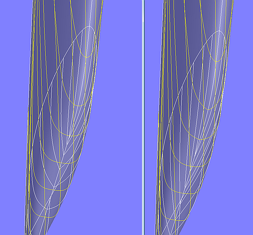
Model fin_keel_tipround.ms2 – effect of curve velocity of SubCurve c0 on the shape of the Blend Surface. Left: c0 with relabel. Right: c0 without relabel
Model fin_keel_tip.ms2 – tip rounding with Blend Surface
2.6 Round transition between keel fin and ballast bulb
In tutorial 10 "Ballast Keels", the model bulb_revolution_surface.ms2 shows another example of how a Blend Surface can be used to easily create a transition between keel fin and a ballast bulb. Since the construction will not be explained further there, it should be made up here.
The base surface of the keel fin is Ruled Surface keel_0, spanned between the Foil Curve root_keel_0 at the keel root and the Foil Curve tip_keel_0 at the keel tip. The ballast body is the Revolution Surface bulb_0, whose meridian curve is the Foil Curve bulb_meridian.
For the rounding Blend Surface keel_fillet we need 4 supports, two snakes on surface 1 and two snakes on surface 2. The first snake on surface 1 is the B-spline Snake sn1; it determines the beginning of the rounding on the keel fin. The second snake on surface 1 is the Intersection Snake sn2, in which keel_0 is cut by the ballast surface bulb_0. This Itersection Snake is projected onto the bulb surface as Projected Snake sn3. The second snake on surface 2, i.e. the one, which defines the end of the fillet on the bulb surface, is the B-spline Snake sn4, generated with 5 control magnets. With these 4 snakes the Blend Surface keel_fillet is determined.
The final portions of keel fin and bulb, which are not covered by the fillet, are created by the SubSurface keel and the SubSurface bulb.
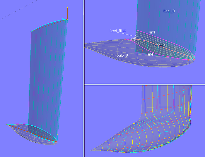
Modell bulb_revolution_surface.ms2 – rounding between keel fin and ballast bulb with Blend Surface (Tutorial 10)
With the property "Type" of the Blend Surface the shape of the fillet can be modified. For Type = 1 the edge joint is tangential, for Type = 2 it is both tangential and continuous in curvature; the fillet is somewhat narrower.
So far to form features.
======================================================================================