The Solve Set Entity
About iterative solutions of geometry problems
by Reinhard Siegel
October 2020
Content
Introduction
The Solve Set Entity
Exercise 1 – maximum curve width
Exercise 2 – maximum hull beam
Exercise 3 – arc touches curve
Exercise 4 – ellipse touches curve
Elliptical bowrounding
Further Solve Set applications
• Proximity Bead - arc touches two curves
• Arc touches curve - version with Proximity Bead
• Hydrostatics - free floating position
• Automated variation of hull form
Introduction
There are geometry problems that are not easy to solve. For example, construct a line that runs through a certain point and is tangent to a circle. Or you can determine the maximum width of a curve or a trunk. You can try to approximate these geometrical constructions manually, but you have to repeat them if the basic geometry changes. MultiSurf offers a permanent, fixed solution for such geometry tasks - the entity Solve Set.
This tutorial was inspired by a MultiSurf user who asked how the waterlines of a boat hull can be rounded elliptically at the bow. The solution to this geometry problem makes it necessary to determine the point of contact between waterline curves and elliptical arcs. In order for this to be a permanent part of the model, a special entity must be used - a Solve Set.
As an introduction to the topic of Solve Sets, two simple examples are considered first. Then it is examined how the center and radius of a circle that touches a curve can be determined. Based on this, the point of contact between an ellipse and a curve is determined in order to then answer the question of the elliptical bow rounding. Finally, two examples are used to show how Solve Set objects can be used to determine the free floating position of a hull and to vary the shape of the hull for target values of displacement and LCB.
Abbreviations used:
cp: control point (support point)
mc: master curve = support curve
cp1, cp2, ...: denotes 1st, 2nd, ... point in the list of supports of a curve. It is not an actual entity name.
mc1, mc2, ...: denotes 1st, 2nd, ... curve in the list of supports of a surface. It is not an actual entity name.
In the following the terms used for point, curve and surface types are those of MultiSurf. This may serve the understanding and traceability.
The Solve Set entity
The Solve Set entity enables geometric constructions that are not possible with the point, curve and surface types available in MultiSurf alone.
Solve Set - characteristic data:
Name -- as with any entity
Layer -- as with any entity
Lock -- as with any entity
Type –- 0 (Dormant) or 1 (Active)
Log Tolerance
No. Free –- Number of solve operations
Entities –- Entities required for solve
User data –- as with any entity
The Solve Set entity requires the objects needed for the solution to be entered in a specific structure:
(1) Free objects with a fixed number of float data: Point, Magnet, Bead, Ring, XPlane, YPlane, ZPlane. Depending on the number of float data, each contributes 1 to 3 degrees of freedom for a total of N degrees of freedom (unknowns).
(2) Constraints. These are N pairs of objects in the pattern ( point, plane/surface). Each pair represents one equality constraint: in the desired final configuration, each point will have zero clearance from its corresponding plane or surface.
At least one object in each target pair must be dependent on at least one of the free objects. Solve Set tries to adapt every free parameter so that all goals (zero distance) are achieved at the same time. This usually requires an iteration. If this iteration converges within the tolerance, the solution operation is successful and all objects involved remain in updated positions.
The Solve Set entity makes its solution a permanent part of the model when Type is set to "Active".
Exercise 1 – maximum curve width
A simple problem – find the position of maximum width of a curve.
Manual solution
Let us consider the model curve_bmax_manual.ms2. Where is the point on curve c0 with maximum distance from the centerplane? The manual solution would be this: one places the Bead e0 on the curve c0 and moves it. The Y-value is shown in the coordinate display in the Status Bar.
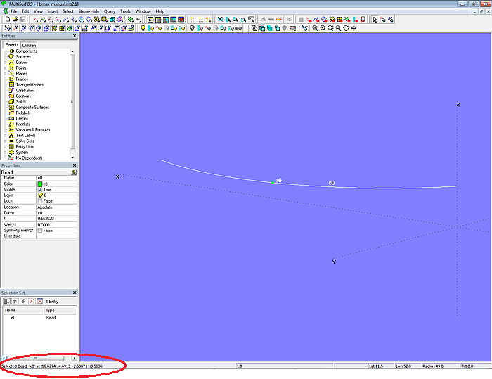
Model curve_bmax_manual.ms2 - determination of the maximum width with Bead e0 and Status Bar
When the shape of curve c0 is changed, the position of e0 must be redefined.
Solution with Solve Set
In model curve_bmax_solveset.ms2, however, the position of e0 at maximum width is automatically determined. The Solve Set entity is used for this purpose.
Let us take a closer look at the model. There is curve c0. The Bead e0 lies on c0. It is support for the Tangent Point tp. The 2-point Plane a0 is defined with e0 and tp. It is therefore the normal plane of curve c0 at curve point e0. There is also Point p1, which is offset from e0 in Y-direction only.
The object list of the Solve Set solve_bmax_curve is: {e0; p1; a0}. This means: the Solve Set should move the free object Bead e0 so that the distance between Point p1 and 2-point Plane a0 becomes zero.
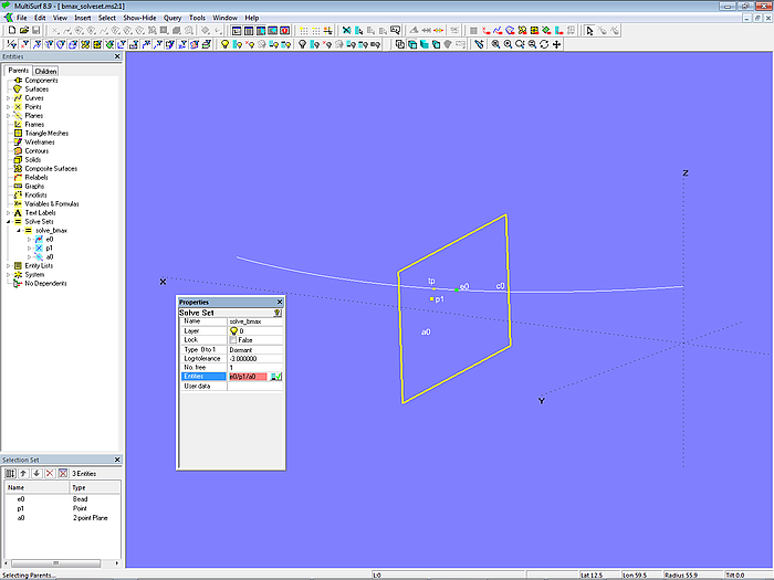
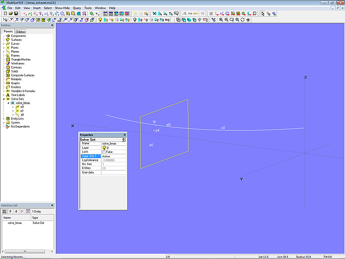
Model curve_bmax_solveset.ms2 - Solve Set solve_bmax_curve inactive (Type = Dormant)
If e0 is in front of the maximum width, p1 is behind plane a0:
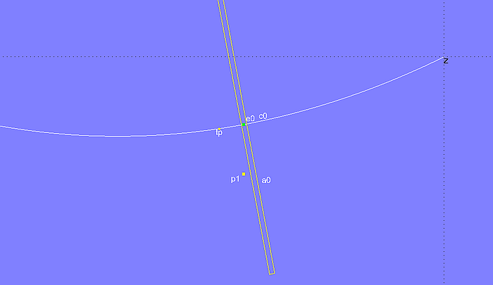
If e0 is aft of the maximum width, p1 is in front of plane a0:
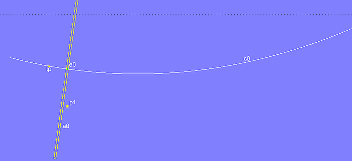
If p1 is at zero distance from a0, then e0 is at the maximum Y-position. Exactly this point is determined in model curve_bmax_solveset.ms2 by Solve Set solve_bmax_curve with its list of free object and pair of constraints: {e0; p1; a0}.
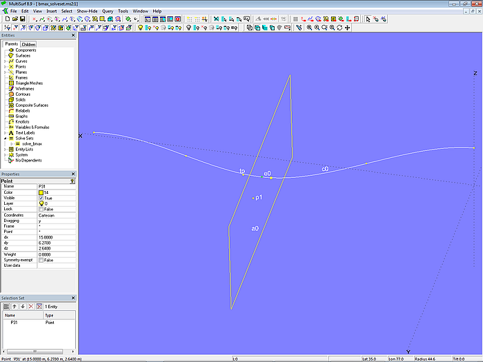
Model curve_bmax_solveset.ms2 - Solve Set solve_bmax_curve active; the position of greatest width is automatically found for Bead e0.
If the curve shape is changed, e0 automatically moves to the position of maximum width.
Model curve_bmax_solveset.ms2 - if the Solve Set is active, its solution is a permanent part of the model.
Exercise 2 - maximum hull beam
Finding the widest part of a boat hull is a little more complicated. There are two search directions here – lengthways and vertical.
Manual solution
With model hull_bmax_manual.ms2, the solution can only be found manually by moving the Magnet m0. It is not necessarily the case that the greatest width of the hull occurs at deck side. The hull cross section could show some tumble-home.
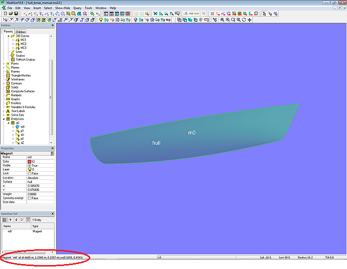
Model hull_bmax_manual.ms2 - manual determination of maximum beam position with Magnet m0 and Status Bar
Solution with Solve Set
In model hull_bmax_solveset.ms2, on the other hand, the problem is solved by the Solve Set entity solve_bmax_hull.
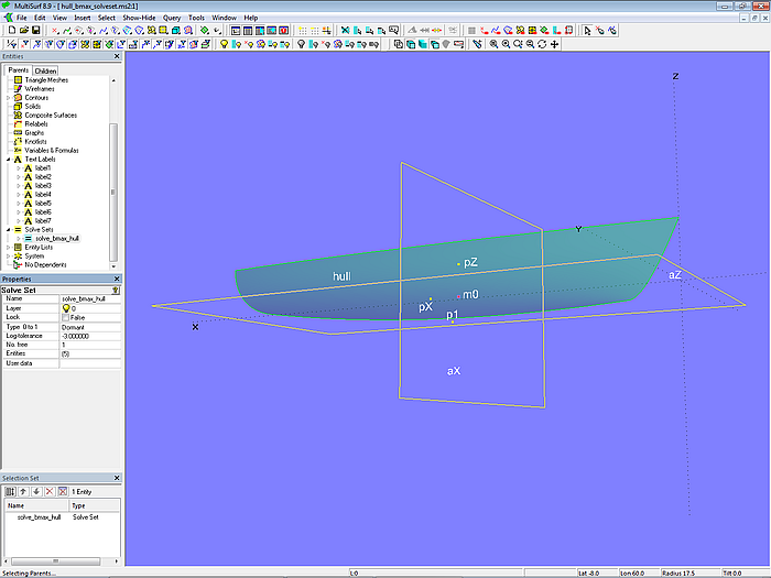
Model hull_bmax_solveset.ms2 - Solve Set solve_bmax_hull inactive
Magnet m0 lies on the hull. Relative to m0 lie Point pX, which is offset in X-direction, and Point pZ, which is offset in Z-direction. Dependent on m0 is also the Offset Point p1 (it is perpendicular to the hull surface). Magnet m0 and Point pX determine the 2-point Plane aX (station plane), while m0 and Point pZ define the 2-point plane aZ (waterline plane).
The Solve Set solve_bmax_hull operates with this list of free object and pairs of constraints {m0; p1; aX; p1; aZ}. This means that the u- and v-parameter values of the free object m0 are determined by iteration in such a way that p1 has a distance of zero from both aX and aZ (pair 1 and pair 2 of constraints), that is, m0 lies in both planes. Then m0 is at the maximum beam position on the hull surface.

Model hull_bmax_solveset.ms2 - Solve Set solve_bmax_hull active
Note: Exercise 1 and Exercise 2 can also be solved with the point types Proximity Bead, Proximity Ring and Proximity Magnet.
Exercise 3 – Arc touches curve
A waterline that ends at the bow with a certain width should be rounded off by an arc. It is known where the arc begins. Find the position of the center point (and thus the radius) so that the arc touches the waterline curve. This task is shown in general form in model arc_tangent_to_curve.ms2.
Manual solution
On the one hand there is curve c0, on the other hand Arc c1 (Type = 2). It begins at Point p0, its center point is Bead e1 on Line l0, and it ends on the imaginary line e1-p2.
If e1 is moved, the position of the center of the circle changes, as does its radius, since p0 is fixed. In this way a position of e1 can be found manually at which the circular arc touches the curve.
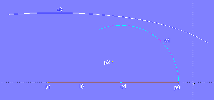
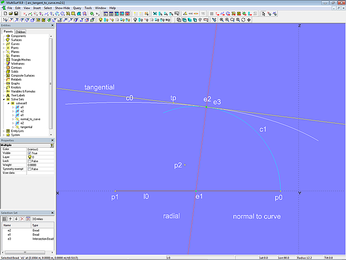
Model arc_tangent_to_curve.ms2 - the position of Bead e1 is to be determined so that Arc c1 touches curve c0. Here the radius (distance p0-e1) is still too small.
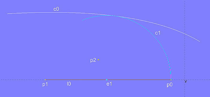
Model arc_tangent_to_curve.ms2 - manually defined position of e1 so that the circular arc touches the curve
If the shape of curve c0 changes, the position of e1 must be corrected. Approaching the solution is acceptable if you only have to do it once or twice in the model. However, if the contact with the curve by the circular arc is to be a permanent property of the model, a Solve Set entity must be used.
Solution with Solve Set
What are the geometric conditions for curve c0 to be touched by Arc c1? Obviously, the distance between a point on the circle and a point on the curve must be zero. In addition, the tangent in the circle point must be the same as the tangent in the curve point. Equivalent to this is: the normals have to be the same.
In a circular arc, the normal always passes through the center; the tangent is perpendicular to it.
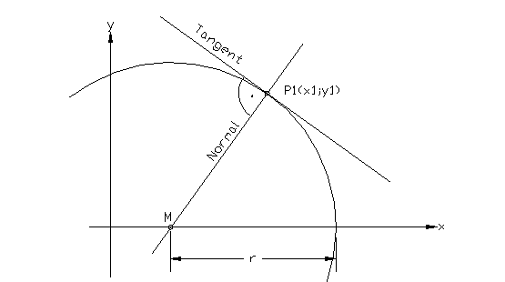
Circle - the normal passes through the center.
In order to incorporate these conditions into the model arc_tangent_to_curve.ms2, there is Bead e2 on Arc c1. Tangent Point tp_e2 is dependent on this. The 2-point Plane radial is defined with both points. This plane intersects curve c0 in the Intersection Bead e3. The Tangent Point tp_e3 is dependent on e3. The 2-point Plane normal_to_curve is generated with e3 and tp_e3. It is the normal of curve c0 in point e3. This plane intersects Line l0 in Intersection Bead C. With Beads e3 and C the 2-point Plane tangential is defined. It is the tangent of curve c0 in point e3.

Model arc_tangent_to_curve.ms2 - Solve Set solve_touch_curve dormant
The two free objects of the Solve Set solve_touch_curve are the Beads e1 and e2. Their position (their t-parameter values) must be varied in such a way that, on the one hand, e1 has zero distance from plane normal_to_curve (1st pair of constraints). Then plane normal_to_curve will pass through the center of the circle, thus it is also the normal to the circle. On the other hand, e2 must also be at zero distance from the plane tangential (2nd pair of constraints). Then e2 is also at zero distance from e3.
Hence the entities required for solve of the Solve Set solve_touch_curve read: {e1; e2; e1; normal_to_curve; e2; tangential}.
Model arc_tangent_to_curve.ms2 - Solve Set solve_touch_curve active
If the curve c0 is changed, Solve Set solve_touch_curve automatically finds the appropriate center point of the circular arc (Bead e1).

Model arc_tangent_to_curve.ms2 - Solve Set solve_touch_curve inactive
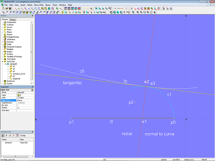
Model arc_tangent_to_curve.ms2 - Solve Set solve_touch_curve active
Exercise 4 - ellipse touches curve
Instead of a circular arc, an elliptical arc should touch a waterline curve. This situation is demonstrated in the model ellipse_tangent_to_curve.ms2.
Apart from the position of the center, there is only one determinant of a circle, the radius. Whereas in the case of an ellipse, there are two shape-determining quantities, the major semi-axis and the small semi-axis. Therefore a relationship between the semi-axes must be specified.
Manual solution
In model ellipse_tangent_to_curve.ms2 there is curve c0. This should be touched by the ellipse c1 (Conic Section, Type = 1. Ellipse). Point p0 defines its main vertex. The segment p0-e1 is the major semi-axis, the small half-axis is the segment e1-p6. The length ratio between the two axes determines Variable b.
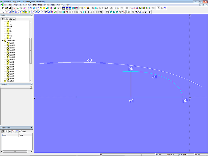
Model ellipse_tangent_to_curve.ms2 – the position of the Bead e1 is to be determined so that elliptical arc c1 touches curve c0. Here its major semi-axis (distance p0-e1) is still too short.
By moving Bead e1 one can manually find the position of the center point at which ellipse c1 touches curve c0.
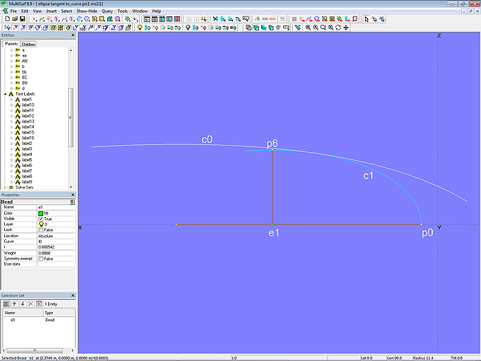
Model ellipse_tangent_to_curve.ms2 - manually determined position of e1 so that the arc of the ellipse touches the curve.
If the contact with the curve by the elliptical arc is to be a permanent property of the model, a Solve Set entity must be used.
Solution with Solve Set
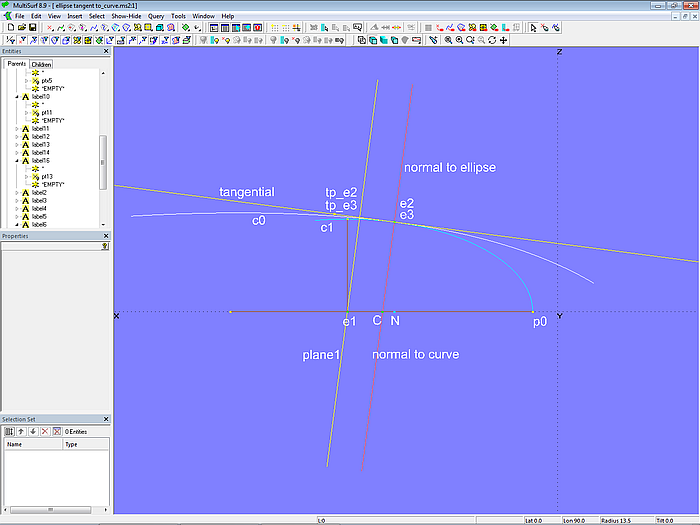
Model ellipse_tangent_to_curve.ms2 is similar to model arc_tangent_to_curve.ms2. Bead e2 lies on the elliptical arc c1 (Conic Section, Type = 1. Ellipse). Tangent Point tp_e2 is dependent on this. With both points the 2-point Plane normal_to_ellipse is determined (normal of the ellipse at Point e2). The plane intersects curve c0 in the Intersection Bead e3. This is support for Tangent Point tp_e3. The 2-point Plane normal_to_curve is defined with both points (normal of curve c0 at point e3). This plane intersects Line l0 in the Intersection Bead C. With e3 and C the 2-point Plane tangential is created (tangent of curve c0 at point e3).

Model ellipse_tangent_to_curve.ms2 - Solve Set solve_touch_curve inactive
With the circle problem, it was the condition for the normal of curve c0 in Bead e3 that it passes through the center of the circle (Bead e1). Then it is also the normal to the circle. In the case of the ellipse problem, however, the normal does not run through the center, but cuts off the subnormal sn on the major half-axis. Therefore there is in addition the Offset Plane plane1, which passes through the ellipse center M(mx; my). It is parallel to the 2-point Plane normal_to_ellipse by the offset value d.
With help of the relationship for the subnormal sn at point P(px; py), the distance d for the Offset Plane plane1 can be calculated.
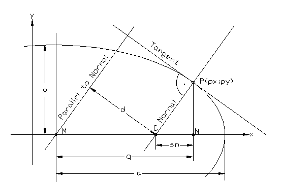
Ellipse - the normal does not pass through the center.
The following applies to the subnormal sn:
sn = b2 / a2 * q
with:
a - length of major semi-axis
b - length of the semi-minor axis
q - distance between point N and center M
The following also applies:
d / MC = PN / PC
with:
MC - distance between point C and center M
PN - distance between points P and N
PC - distance between points P and C
So it follows:
d = PN / PC * MC
MC = q – sn
MC = q (1 – b2 / a2)>/p>
Thus:
d = PN / PC * q (1 – b2 / a2)
The offset value d for the Offset Plane plane1 is calculated with the help of Formula entities.
The free objects of the Solve Set solve_touch_curve are Beads e1 and e2. If the free object Bead e1 has zero distance from Offset Plane plane1 (1st pair of constraints), and at the same time the other free object Bead e2 has also zero distance from the plane tangential (2nd pair of constraints), then the normals match and the curves touch.
Hence the list of entities required for the Solve Set solve_touch_curve is: {e1; e2; e1; plane1; e2; tangential}.
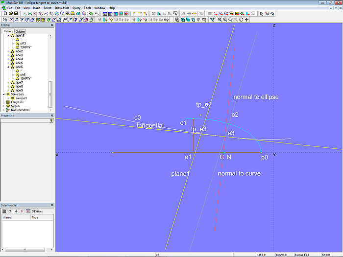
Model ellipse_tangent_to_curve.ms2 - Solve Set solve_touch_curve active
If curve c0 is changed, Solve Set solve_touch_curve automatically finds the appropriate center point of the ellipse (Bead e1).
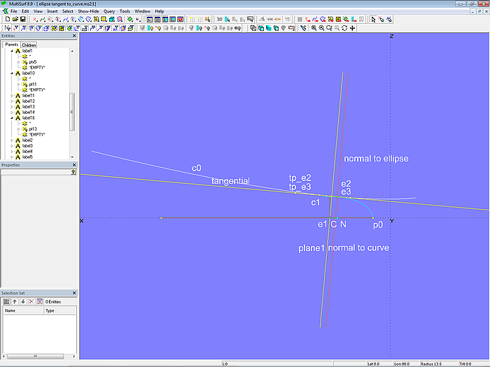
Model ellipse_tangent_to_curve.ms2 - Solve Set solve_touch_curve inactive
Model ellipse_tangent_to_curve.ms2 - Solve Set solve_touch_curve active
Elliptical bowrounding
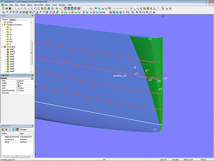
Model sy15-elliptical_bowround.ms2 demonstrates how the stem of a boat hull can be rounded elliptically with the method shown above.
The EdgeSnake n0 runs along the leading edge of the hull surface hull_0. Rings r1 and r2 are located on this snake and determine the SubSnake n1. Ring r0 lies on n1. The waterline at the level of r0 is the Intersection Snake snake_c0. This one should be touched by the elliptical arc c1 (Conic Section, Type = 1. Ellipse).
The structure of the contact construction is basically the same as in model ellipse_tangent_to_curve.ms2, but now snake_c0 and the elliptical arc c1 are parallel to the XY-plane. Ring r0 is projected onto the midship plane as Projected Point p0 and is the vertex of the ellipse. Line l0, on which Bead e1 is based as the center of the ellipse, is dependent on its start point p0.

Model sy15-elliptical_bowround.ms2 - elliptical bowround. Left: Solve Set solve_touch_wl inactive. Right: Solve Set solve_touch_wl active.
The Solve Set solve_touch_wl determines the position of e1 at which ellipse c1 touches the waterline snake_c0. This contact point is Bead e2 on c1, with which the curve part up to the apex is defined by SubCurve c2. Thus the elliptical rounding of the waterline at the level of r0 is found.
If Ring r0 is moved, this entire construction is shifted in the Z-direction and SubCurve c2 will sweep out a surface. The Procedural Surface elliptical_bowround creates this surface.
Model sy15-elliptical_bowround.ms2 - elliptical bow rounding. Solve Set solve_touch_wl is active.
Further Solve Set applications
Proximity Bead - arc touches two curves
Model arc_tangent_two_curves.ms2 shows how two curves can be rounded with an arc of a given radius. For this, the starting point of the circular arc must be the point of contact on one curve, the end point of the circular arc must be the point of contact on the other curve. This requires two free objects that must be positioned so that these conditions are met.
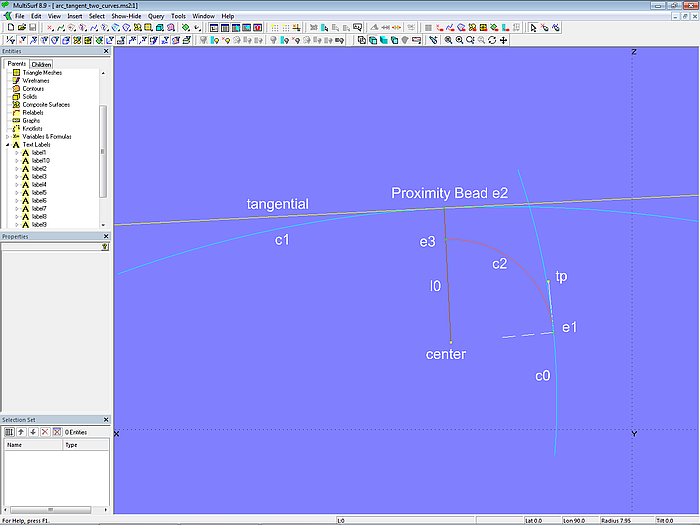
Model arc_tangent_two_curves.ms2 –Circular arc c2 should touch both curves; Solve Set solve_touch_curves not active
Bead e1 (free object 1) is located on curve c0 as starting point of the circular arc. Tangent Point tp and Point px (offset relative to e1 in the Y-direction) depend on e1. With these three points the 3-point Frame frame1 is defined. The X-axis of frame1 points in the direction of the Tangent Point tp, so it is the tangent to curve c0 at point e1. The Z-axis points in the direction of the normal. Point center lies on this Z axis, i.e. the normal, and its dz value corresponds to the radius of the rounding arc.
The end point of the circular arc is point e2 on curve c1. The line center-e2 is the radius line, i.e. the normal of curve c1 at point e2. Consequently point e2 must be positioned in such a way that it has the smallest distance from center (free object 2). With a special type of curve point, the Proximity Bead, this point can be easily generated. A Proximity Bead determines the point on a curve that has the smallest or largest distance from an outside point (depending on the setting).
The free object 2 is therefore determined by the Proximity Bead. In the present case, Proximity Bead e2 must have the smallest distance from Point center. You can also say that Proximity Bead e2 is the base point of the plumb line that is felled from center to curve c1. With the two points center and e2 the 2-point Plane tangential is created, i.e. the tangent of curve c1 at point e2.
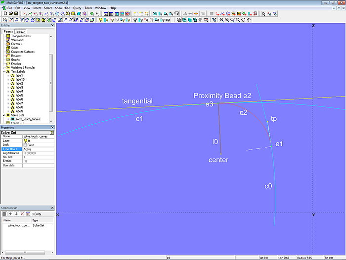
Line l0 connects center and Proximity Bead e2. The Intersection Bead e3 lies on Line l0. It has the distance of the radius of the circular arc from center. With e1, center and e3 this circular arc is generated as Arc c2 (Type = 2).
We are now looking for the position of e1 in such a way that the distance between e3 and the tangent tangential is equal to zero, i.e. Arc c2 touches curve c1. The Solve Set solve_touch_curves is used to determine this position. The free object is Bead e1, the pair of constraints is e3 and tangential. Hence, the list of objects required for the solution of Solve Set solve_touch_curves is: {e1; e3; tangential}.
Model arc_tangent_two_curves.ms2 - Solve Set solve_touch_curves active; Arc c2 touches both curves.
If the shape of the curves changes, the Solve Set object automatically finds the new center point of the rounding arc as well as its start and end point. The same applies to changing the radius of the rounding.
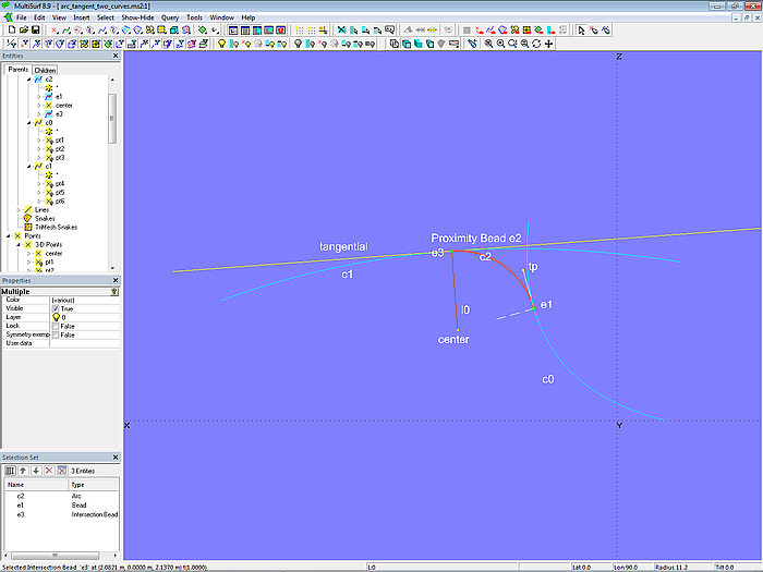
Model arc_tangent_two_curves.ms2 - Solve Set solve_touch_curves active; Arc c2 touches both curves.
Although the construction shown here can also be carried out without a Proximity Bead, its use makes the model simpler and clearer. With the Proximity Bead, one of the two free objects is automatically determined.
Arc touches curve - version with Proximity Bead
How exercise 3 - arc touches curve - can be simplified with the object Proximity Bead is shown in model arc_tangent_to_curve-Proximity_Bead.ms2. It can be clearly seen that the model requires fewer objects.
Center of the circular arc c1 is Bead e1 (free object 1). Proximity Bead e2 on curve c0 depends on this; it has the smallest distance from e1 (free object 2). Line l1 connects e1 and e2, it is the radius line of the circular arc and thus the normal of curve c0 at point e2. With the two points e2 and e1, the 2-point Plane tangential is created, i.e. the tangent of the curve c0 at point e2. Arc c1 intersects Line l1 in the Intersection Bead e3.
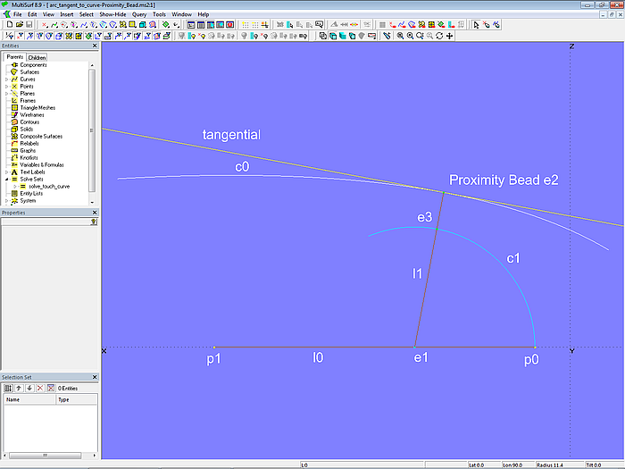
Model arc_tangent_to_curve-Proximity_Bead.ms2 - Solve Set solve_touch_curve not active
The position of e1 and thus the radius (= distance p0-e1) must be selected so that the distance between e3 and the tangent tangential is zero, i.e. Arc c1 touches curve c0.
The Solve Set solve_touch_curve is used to determine this position. The free object is Bead e1, the pair of constraints is e3 and tangential. The list of the objects of the Solve Set solve_touch_curve required for the solution is thus: {e1; e3; tangential}.
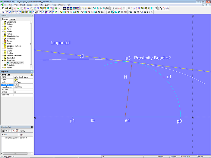
Model arc_tangent_to_curve-Proximity_Bead.ms2 - Solve Set solve_touch_curve active
Hydrostatics - free floating position
In tutorial 14, “How to created computing MultiSurf models”, the model Hydro_free_floating.ms2 shows in detail how the Solve Set entity can be used in combination with Hydrostatic Reals to find the floating position of a boat hull for given weight and center of gravity. For this purpose, the Solve Set entity solve_free_float systematically changes sink and trim until there is a balance between forces and moments of weight and buoyancy.
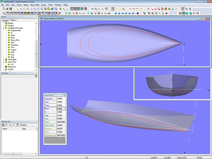
Model Hydro_free_floating.ms2 - free floating position with balance of weight and buoyancy
In model Hydro_free_floating.ms2 the free floating position can also determined when heeling. This makes it possible to assess the asymmetrical shape of the waterlines or to answer the question whether the transom remains clear of the water surface or is already immersed. Heeling with fixed sink and trim leads to incorrect results, since the displaced volume increases. To get realistic answers, the boat must float freely when it is heeled.
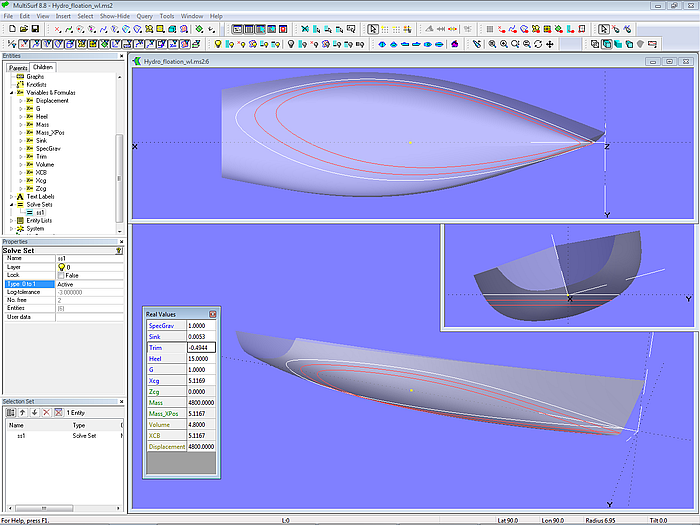
Model Hydro_flotation.ms2 - free floating position when heeling
Automated variation of hull form
Tutorial 16, “Automated variation of hull form”, deals with the problem that when designing a hull shape the point will be reached when the form corresponds to the ideas, but there could be a little bit more displaced volume, and maybe an LCB a few centimeters closer to the stem would be good too (for example). Then the control points of the master curves have to be shifted by a few millimeters here and there, and in addition to the hydrostatic values, the fairness must also be constantly checked. This fine-tuning is time consuming.
The approach described in tutorial 16 makes it possible to automatically derive new master curves from the master curves of an existing hull in order to achieve target values for volume and LCB. Surface fairness, hull outline and shape character of the Mcs are retained.
In model formvariation_model-4.ms2, the Solve Set solve_V_LCB is used to automatically adapt the displacement curve for the derived Mcs so that volume and LCB of the derived hull take given target values.
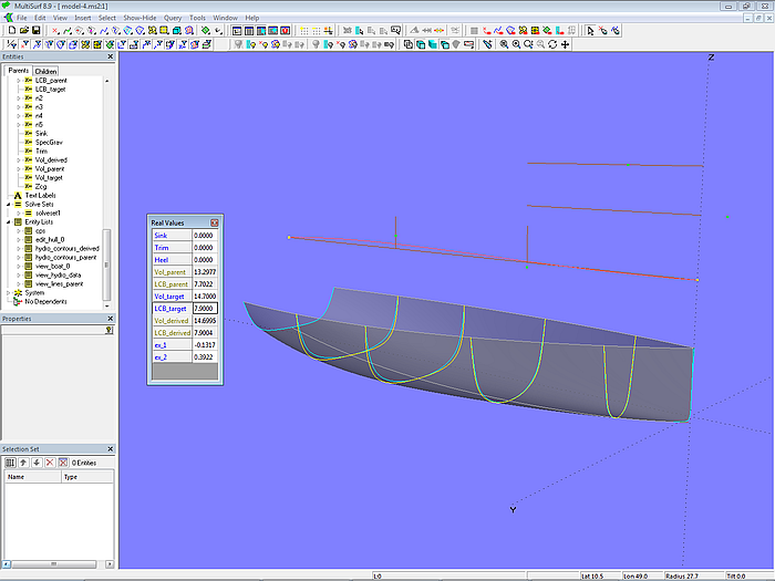
Model formvariation_model-4.ms2 – increased volume and LCB moved aft
======================================================================================