Modeling a Rudder in MultiSurf

Strategies and methods

by Reinhard Siegel

Introduction

This article presents several methods how to create a rudder. It is not about designing a rudder of specific dimensions and shape, but shows what methods are available and which strategy is practical for your purpose.

Abbreviations used:

cp: control point (support point)
mc: master curve (support curve, control curve)

Cp1, cp2, mc1, mc2 etc are not the names of distinct point or curve entities, but denote an object in a general sense, for example cp1 as being the first parent point of a Foil Curve or mc1 as being the first master curve in the sequence of parent curves for a lofted surface.

In the following the terms used for point, curve and surface types are those of MultiSurf. This may serve the understanding and traceability.

1. Foil Curve

Airfoils are widely used in designing hull appendages. In MultiSurf one can select for the curve type Foil Curve from 5 standard NACA foil families and user defined foils (imported via the utility FOILFIT; see section 7).

A Foil Curve with 3 control points (cp1 = start point, cp2 = thickness, cp3 = end point) is one half of a symmetric foil, it lies in the plane of its 3 cps. and for the time being we will restrict to this standard shape.

With thickness we refer to the maximum thickness of the half section, not local thickness or distribution of thickness along the chord of the Foil Curve.

For Foil Curves only the distance of the thickness cp from the chord line counts, its fore-and-aft position is immaterial.

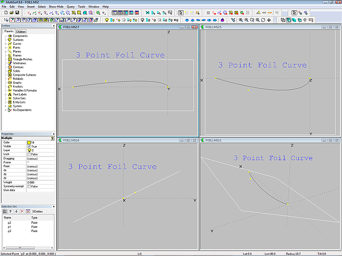
Foil Curve defined by 3 control points: start, thickness, end. Result is one half of a symmetrical foil. The curve lies in the plane of its control points.

2. Surface Types for Rudder Design

2.1 C-spline Lofted Surface

The C-spline Lofted Surface is a standard type used for the design of hulls. Let us see how we can also use it for a rudder (model rudder-cloft.ms2). In opposition to a hull surface the mcs are no freeform curves, but Foil Curves. Their control points define in spanwise direction the trailing edge, the leading edge and the thickness curve. In order to achieve a fair rudder surface those curves must be fair spanwise curves – the principle is the same as in hull surface modeling.

First the leading edge and trailing edge are created as C-spline Curves. This determines the number and location of cps, which are required to get the intended shape of the rudder planform. In the example model cloft-1.ms2 6 cps are used. This is no dogma; if the planform is a trapeze, just 2 cps per curve would do. The most complex curve is decisive. When leading and trailing edge are established, corresponding cps are connect by lines, so we get the chord lines of the foil section. Now a line is run from the mid point of cl_rt (chord of root section) down to the midpoint of cl_tp (chord of tip section). This Line l0 intersects the chord lines of the inner sections (cl_2, cl_l3, cl_4, cl_5) in the Intersection Beads e_2 to e_5.

Now we can create the thickness cps (points th_rt, th_2, th_3, th_4, th_5, th:tp) which are made relative to the chord line beads. Setting dx = dz= 0 the dy values of these cps define the half thickness of the foil sections. The dragging of the thickness cps to is restricted to the y direction only, thus all defining points of a section mc will be in a common plane.

Next run a C-spline Curve through the thickness cps. This guiding curve visualizes the spanwise distribution of thickness.

Note, that for a Foil Curve only the distance of the thickness cp from the chord line counts, its fore-and-aft position is immaterial. Since all the thickness cps are relative to beads on Line l0, the thickness curve th bends only normal to the center plane, what is convenient for its fairing.

Now let us make the mcs as Foil Curves using the corresponding points of trailing edge, thickness curve and leading edge. Finally span a C-spline Lofted Surface across the mcs.

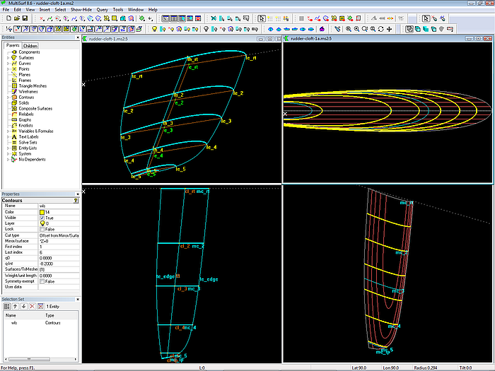
Model rudder-cloft.ms2: C-spline Lofted Surface on 6 Foil Curve mcs.

The construction to fix the thickness cp on a bead residing on the chord line ensures, that the Foil Curve is straight in Y-view. This also allows to orient a mc to the presumed direction of the water flow over the rudder surface. Thus the water “sees” the section shape selected for the mc.

A C-spline Lofted Surface rudder also makes it possible to use different types of Foil Curves for the mcs. Thus, for example, Naca section of 63 series mcs at the root can be blended into mcs of the 65 series at the tip.

2.2 Procedural Surface

A rudder surface could also be looked at as being the path in space of a foil section, that moves spanwise from root to tip. At each position the foil starts at the trailing edge, ends at the leading edge and takes its half thickness from a thickness distribution curve. This kind of surface can be constructed in MultiSurf by a Procedural Surface.

The construction has several advantages:

any kind of curve can be used for mcs
complex curved mcs can be mixed with simple curved ones
no effect of unsimilar t distribution of mcs on section shape
moving foil section can change orientation with respect to flow along span

In the model rudder-procsurf.ms2 the leading edge mc is a B-spline on 6 cps; note the tight bend at the root; B-splines are “soft” and bend easily with relative few cps. The trailing edge mc is an Arc (simple,no fairing), the thickness mc is a C-spline Curve on 5 cps (stiff, little fairing). The moving curve is the Foil Curve c0. Its start cp is the bead e_te on the trailing edge curve. Both thickness curve and leading edge are intersected at the height of e_te to get thickness cp and end cp.

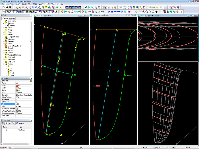
Model rudder-procsurf.ms2. The trailing edge is an Arc, the thickness curve a C-spline, the leading edge a B-spline Curve. Moving curve is Foil Curve c0. No effect of unsimilar distribution of t parameter along mcs on section shape.

2.3 Foil Lofted Surface

MultiSurf also offers the surface type Foil Lofted Surface which is convenient for appendage design.

In a Foil Lofted Surface master curves (mcs) are planked by Foil Curves: on each of the mcs MultiSurf locates points at the same parameter value t, then uses the resulting series of points as the control points for the Foil Curve. When mc1 defines the trailing edge, mc2 the spanwise variation of thickness and mc3 the leading egde, we get one half of a symmetric foil-lofted surface.

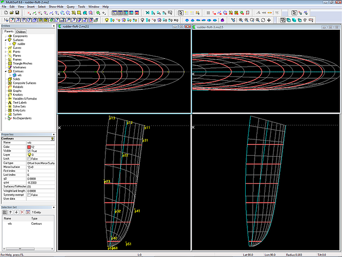
Model rudder-floft.ms2 shows a Foil Lofted Surface based on 3 spanwise mcs. Each mc is a B-spline Curves of equal degree. The number of cps is also equal for each mc. Further corresponding cps are positioned at the same z coordinate.

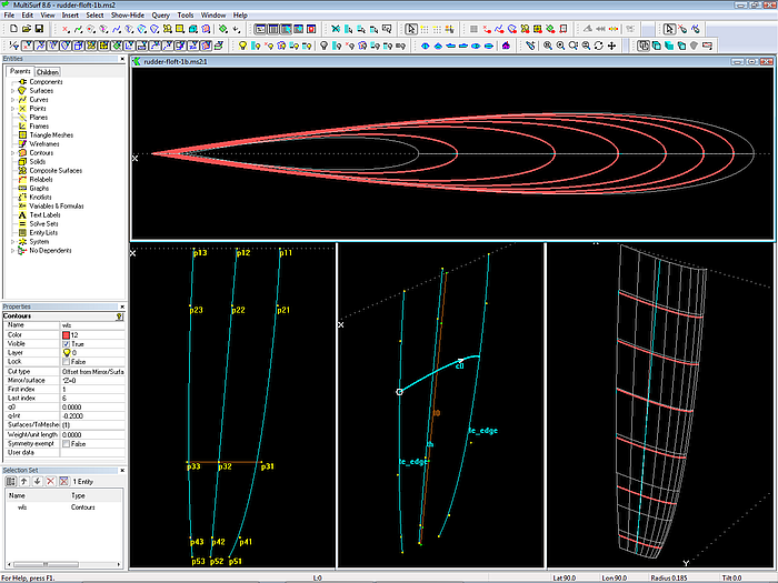
Model rudder-floft.ms2: Foil Lofted Surface; trailing edge, thickness distribution and leading egde mcs are B-spline Curves of same degree, same number of cps and z coordinates of corresponding cps alike.

U-parameter curves and form effects

In the previous example the construction underlies several restrictions. The number of cps is determined by the most complex curve required to form it. When the leading edge needs 7 cps to form it to your wish, you must also use 7 cps for trailing edge and thickness curve. Further the corresponding cps must be aligned.

What happens if you do otherwise is illustrated in the next figure. Here the trailing edge is an Arc, the thickness curve a C-spline and the leading edge a B-spline. This dissimilarity in the setup of the model severely hurts the waterline shape.

Foil Lofted Surface: trailing edge mc is Arc, leading edge mc is B-spline, thickness mc is C-spline. Left image: unsimilar t-distribution along mcs hurts the section shape.Right image:leading edge and thickness mcs relabeled equally to trailing edge using Procedural Curves.

Note: The u-parameter curves of a Foil Lofted Surface must be straight in profile view, otherwise the section shape is unfair.

The run of the u-parameter curves depends on the labeling of the mcs (think of each point of a curve as being labeled by a specific value of t). Although t is equal at each mc, the actual location of the corresponding cps can be different in span direction.

To achieve straight u-parameter curves the labeling of the mcs must be similar.

How to avoid unsimilar labeling

Use B-spline Curves of equal degree, equal number of cps and put corresponding cps to equal z coordinates. This method is demonstrated in model rudder-floft.ms2.

Use X-spline Curves. Mcs must start at the same z coordinate, also all end points must have equal z values. Otherwise the number of cps for each mcs can be different.

X-spline Curves are stiff; a tight curvature will need several closely spaced cps, carefully positioned to avoid unfairness. B-spline Curves are “soft”, easy to freeform.

How to control curve labeling

MultiSurf also offers means to control the labeling of any curve type, for example by the curve types Procedural Curve and SubCurve. The relabeling of a mc by a Procedural Curve is superior, as it automatically adapts to changes in the t parameter distribution of the curve, from which the labeling is taken, as well as it adapts to form changes of the curve, whose labeling it replaces.

With a SubCurve its beads must be repositioned when the host curve is modified, in order to keep the u-parameter curves of the Foil Lofted Surface under control.

3. Thickness mc

Display of t/c ratio

The thickness of a foil section is typically expressed in percentage of chord line length. However, for its thickness cp the Foil Curve requires a distance from the chord line. Say, with a 3 point Foil Curve the cp has got a dy of 0.025 m, than the full thickness of the section is 0.05 m. If we want to know what t/c ratio this is, we need section chord length and a calculator.

A display of t/c values is thus helpful. This is easily done in MultiSurf with a set of Formula entities. Open again model rudder-cloft.ms2. In the Entities manager select the Entity List view_data, then choose from the main menu Tools/ Real Values to open the Real Values dialog window. It lists chord line length (c1 –c6), half thickness (ht1 – ht6) and thickness ratio (tc1 – tc6) of each Foil Curve mc.

This are the formula expressions for the root mc:

with
start point: te_rt
thickness point: th_rt
end point: le_rt

than
chord length: c_rt = DIST(le_rt. te_rt)
root half thickness: ht_rt = DIST(th_rt, e_rt)
root thickness ratio: tc_rt = 2* ht_rt / c_rt

The data for the other mcs are calculated accordingly. Drag a point and see how the Real Values in the dialog window change.

Further there is a graph, that shows how t/c changes along span – a curve shows more than a set of numbers. To display it select the Entity List view_tc_graph, then click the Show Parents button.

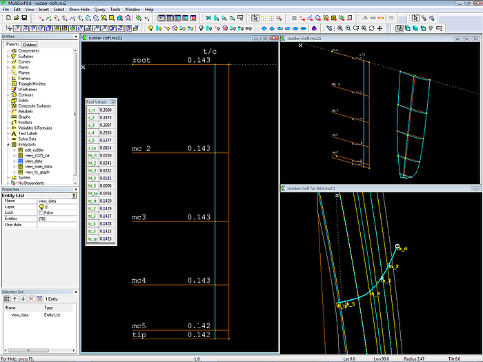
Model rudder-cloft.ms2: Formula entities calculate chord length, thickness and thickness ratio for the Foil Curve mcs. Left image: Real Values display and graph of t/c ratio. Bottom right: 3D view of thickness curve is helpful for fairing.

Thickness control with Procedural Surface

In model rudder-6.ms2 the thickness ratio curve itself is used to control the section thickness. The surface type is a Procedural Surface, moving curve is a Foil Curve, which gets its cps from a C-spline trailing edge, a C-spline thickness curve and a B-spline leading edge curve. For the 6 spanwise sections the thickness ratio can be edited directly by moving the t/c points in the graph. The t/c ratio is translated into section thickness values for the definition of the thickness curve.

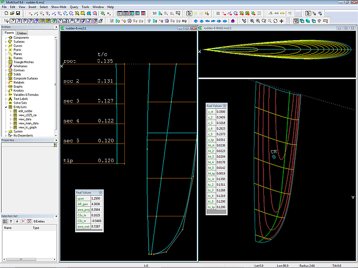
Model rudder-6.ms2: Procedural Surface - moving curve is Foil Curve, which gets its cps from C-spline trailing edge mc, C-spline thickness curve and B-spline leading edge curve. Left image: the thickness ratio, which can be edited directly in the graph, is translated into section thickness values for each spanwise section. Right image: shows section data, centroid of area and quarter chord line.

4. Geometrical dimensions

Model rudder-cloft.ms2 and rudder-6.ms2 include apart from Real Values of section data also Real Values of main geometrical dimensions of the rudder. Select the Entity List view_main_data, then Tools/ Real Values. Span, geometrical aspect ratio, wetted surface (both sides), area (projected on centerplane) and the location of its centroid are displayed. c_CA is the length of the chord passing through the centroid CA of the projected area, h_CA the distance to the root chord. Those data are of use for the scantling calculation of rudder stock and bearings.

The Entity List view_c025_ce holds the quarter chord curve and the centroid CA. Select the list, then click the button Show Parents.

5. Tip shape

A look at the tip section of our model rudder-cloft.ms2 shows, that the rudder is not closed at the tip. Also, the rudder needs a more rounded forefoot; we left this aside when modeling the leading edge. In other words, a tip rounding is required.

Model tip round.ms2 demonstrates the principle, which follows almost the model wingtip2.ms2 from the MultiSurf Examples folder. First, the tip is closed by the Ruled Surface tip_flat, spanned between the mc at the tip and a portion of its chord line (SubCurve c0). Then the Blend Surface entity is used to provide the smooth local blending between the rudder surface and tip_flat.

A Blend Surface is defined by four snakes — two on each of the basis surfaces. The first snake on the rudder surface is the Intersection Snake sn1; cutting object is the 3-point Plane plane1. The second snake sn2 on the rudder surface is the EdgeSnake along the tip. The third snake sn3 is the EdgeSnake of the Ruled Surface tip_flat, which joins the rudder tip edge. And finally the fourth snake sn4 is the inner edge of tip_flat.

Moving the cutting plane controls the start of the tip rounding. Moving the beads tip1 and tip2 controls the round off at front and rear. These two beads define the SubCurve c0, parent for the Ruled Surface tip_flat. Note, that c0 is relabeled in a specific way; if this is ommited, the Blend Surface will have unwanted folds or grooves.

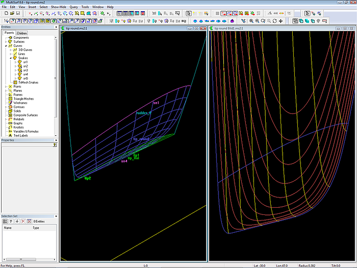
Model tip round..ms2: Blend Surface used to round off the tip of the rudder.

6. Examples

Standard rudder

In model rudder-on-full-chine-sy2.ms2 a relative of the C-spline Lofted Surface rudder example is added to a 12 m sailboat hull. There is also a rudder stock. Normal to it is the small planar surface st_plane, which is used to intersect rudder surface and stock. So one can check if the stock is inside the rudder surface.

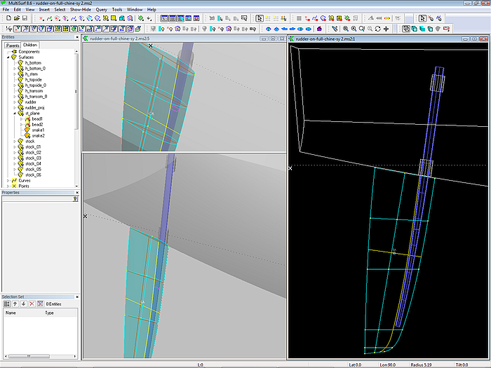
Model rudder on full chine sy 2.ms2.

Twin rudder with cambered foil section

In the rudder models that were discussed so far, the foil sections used are one half of a symmetrical section. A rudder with cambered full sections is demonstrated in the model twin rudder.ms2.

The whole construction is based on a 3-point Frame. The planform is a trapeze, so a Foil Curve mc for the root and another one for the tip are all we need to define. A Ruled Surface is spanned between them, and with its intersection snakes against hull and span end the SubSurf rudder is cut off.

The Foil Curves at root and tip use 5 cps: the first point is at the start and the third point at the end of the chord line; the second point and fourth point determine thickness and camber. There is a variable for the camber ratio f/c and a variable for the thickness ratio t/c. By the help of 4 Formual entities those second and fourth points are calculated for root and tip section.

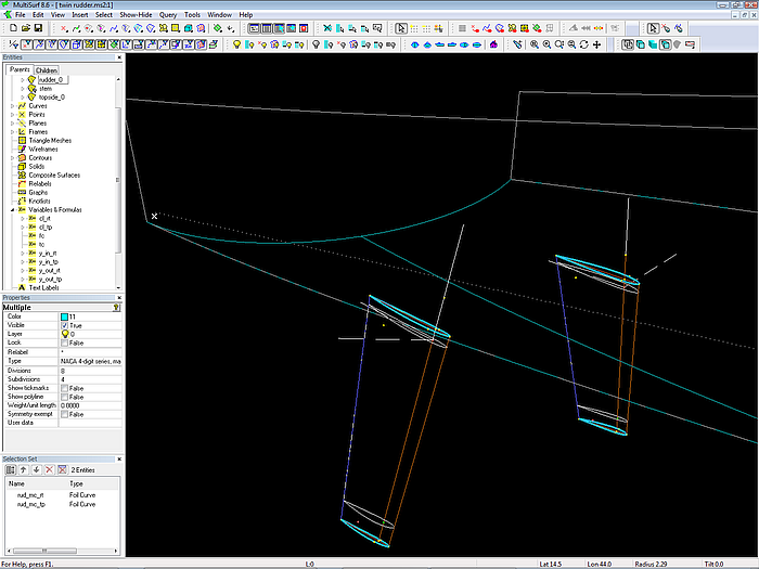
Model twin rudder.ms2: Root and tip mcs of the trapeze rudder are cambered full Foil Curves.

7. FOILFIT 2.01

Apart from the 5 standard NACA foil families MultiSurf supports user defined foils in the definition of Foil Curves. FOILFIT is a utility to create files is in the required format.It fits B-spline parametric curves to arbitrary airfoil and hydrofoil sections. It reads an input data file containing thickness and camber offsets and writes an output file containing B-spline control points. The output file is in the format required for MultiSurf.

FOILFIT version 2.01 runs under Windows XP and higher.

The input file is an ASCII text file in three sections:
(1) The first line is an identifying message for the file.
(2) The second line is an integer telling how many lines follow.
(3) The balance of file is data lines.

Each data line needs four numbers, separated by spaces, free format; all four values expressed as % of chord (see example below):
X-position
thickness function ordinate
thickness function delta
camber function

The thickness function delta is an optional correction to the thickness; if there is no correction to make, use zero in this column. In the following example, the .100 trailing edge thickness is removed by using deltas of .100 (x/c)4.

When fitting a symmetric section (no camber), the camber column can be all zeroes. However, the resulting section will have no camber when used as a 5-point foil in MultiSurf, even if its 2nd and 4th control points are unsymmetrically located.

Example input file (0010-65.dat)

data for 0010-65 foil p. 319 w/ 64 mean line p. 385

17
0.000 0.000 0.000 0.
1.250 1.467 0.000 0.369
2.500 1.967 0.000 0.726
5.000 2.589 0.000 1.406
7.500 2.989 0.000 2.039
10.000 3.300 0.000 2.625
15.000 3.756 0.000 3.656
20.000 4.089 0.000 4.500
30.000 4.578 -0.001 5.625
40.000 4.889 -0.003 6.000
50.000 5.000 -0.006 5.833
60.000 4.867 -0.013 5.333
70.000 4.389 -0.024 4.500
80.000 3.500 -0.041 3.333
90.000 2.100 -0.066 1.833
95.000 1.178 -0.081 0.958
100.000 0.100 -0.100 0.000

FOILFIT uses least-squares fitting with B-spline basis functions. The number of control points is user-controlled (default 8). The B-spline order (4 = cubic), and the control point abscissas are hard-wired. The abscissa control point values are chosen to produce a parabolic (approximately half-cosine) distribution of X vs. t.

Separate root-mean-square error values for thickness and camber fits are displayed as a fraction of chord. For the five built-in foil families, using 8 control points, these ranged from .00001 to .00032, average about .00015. Be sure to examine the screen tabulation of fit - data differences to identify bad data points.

In general, the closeness of fit should improve with increasing number of control points. Fairness, on the other hand, often is compromised by larger numbers of control points. We always prefer to use a small number for fairness, and would increase the number of control points beyond 8 only if we judged the fit to be insufficiently close.

Output file
Like the input file, the output file is in three sections (see example below):

(1) The first line is a verbatim copy of the identifying message.
(2) The second line is two integers:
the number of control points
the B-spline order (e.g., 4 = cubic)

(3) The balance of file is data lines, each with 3 numbers:
abscissa
ordinate for thickness function
ordinate for camber function

All three values are normalized to the range 0 to 1.

The fitted thickness is a B-spline using (x, yt) as control points. The fitted camber is a B-spline using (x, yc) as control points. (Both B-splines use uniform knots.)

The output file takes the name of the input file, with .FOI extension. The output file will generally have to be renamed to be recognized by MultiSurf, e.g. TYPE101.FOI, etc. — we renamed the example file below TYPE165.FOI.

Example output file (made from the above example input)

data for 0010-65 foil p. 319 w/ 64 mean line p. 385

8 4
0.00000 0.00000 0.00000 (Note: this line is required.)
0.00000 0.19834 0.00370
0.02667 0.50750 0.13320
0.14667 0.77953 0.65787
0.34667 0.97395 1.08315
0.62667 1.06479 0.93092
0.86667 0.62715 0.45153
1.00000 0.00000 0.00000