Fitting Surfaces to Predefined Shapes
How to create a MultiSurf model from a paper lines plan
by Reinhard Siegel
Introduction
When you create a new design from scratch, you have complete freedom to shape the surfaces, and when all looks pretty and satisfies the design parameters you can quit. This is "freeform design". But if the objective is to reproduce a predefined shape it comes to “surface fitting”. The freedom to shape is replaced by the challenge to create a geometry which is close to the given data as well as being fair. In this article we will discuss the required steps how to savely overcome this exercise in MultiSurf.
It is certainly an advantage if you have knowledge of the behavior of the various kinds of curves and surfaces, which are available in MultiSurf. What is ok for a slender sailing yacht hull does not work for a powerboat or a container vessel with its flat side and bottom. You are the master of the fitting process, you must decide what surface and curve type is suitable, and where all those supporting master curves and their control points have to go.
Abbreviations used:
cp: control point (support point)
mc: master curve = support curve
In the following the terms used for point, curve and surface types are those of MultiSurf. This may serve the understanding and traceability.
1 - Fitting means comparison - casting the graphical data into numerical form
The fitting process requires a permanent comparison of the given geometry against the created computer model. For this purpose MultiSurf offers the entity Wireframe. A WireFrame presents the content of a .3DA file (3D ASCII Drawing File). A .3DA file contains XYZ-coordinates of points in ASCII format. The Wireframe entity displays the 3DA file by a polyline passing through its points. It cannot be used in the construction of other MultiSurf entities. It is included in a model primarily for display.
A 3DA file can be created in several ways:
- translate the lines plan into DXF
- type point coordinates into .3DA format using Windows Notepad (or other)
- import a table of offsets
Method 1: translate the lines plan into DXF
Step 1: create a picture file
First we need to “get the paper picture into the computer”. One possibility is to scan the drawing using a printer-scanner-copy device. Another way is to take a photo with a digital camera. In both cases the result will be a picture file, typically in the popular JPEG format.
As an example let us recreate the hull of the sailing yacht Dorade (design Sparkman & Stephens; 1929). Its set of lines is presented in the book Yachts classiques (Gilles Martin-Raget (text, photos), François Chevalier (drawings); Paris: Editions du Chêne-Hachette Livre, 1998).
When the scan or photo is done load this initial picture into Windows Paint (or any other graphic editor) and save the body plan (stations) and the profile view (hull outline) into two separate files: body_plan.jpg and profile_view.jpg. These files must be digitized.
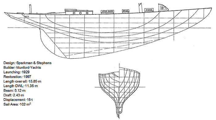
Dorade – profile view and body plan (scan from the book Yachts classiques)
Step 2: Digitize the picture
Now the picture (the lines plan) is “in the computer”, but it consists of pixels. What looks like a red curve on a white background is a band of red pixels embedded in a sea of white ones. The pixel graphic (or raster image) must be transformed into vector graphic, i. e. into lines, polylines, arcs, etc. There are two ways to achieve this:
- automatic vectorization by an utiltity program
- do it yourself – redraw lines manually
Vectorization by an utiltity program
There are image manipulation programs available which can vectorize pixel graphics. An automatic process “redraws” the content of the picture. The result can be saved in various file formats, for example as DXF. This file type is of importance for our purpose as MultiSurf can imported it.
An automatic process has no “feeling” what content of the image is important. Either some edit work is necessary prior to the vectorization or when it is finished. Otherwise a good compromise between accuracy and simplicity cannot be obtained.
It is certainly worthwhile to evaluate the variety of such tools since raster image vectorization can save time for an experienced user. Some process also PDF files.
Redraw lines in a Cad program
If the redraw is done manually in a Cad program it is up to the user which curves of the lines plan are selected and which are ignored. He also can immediately decide which one of the crossing curves belongs to which station when retracing a crowded body plan. So redrawing lines by hand in a Cad program is not that bad as it might sound at first sight. Let us consider this path in the following.
Usually standard Cad programs can paste pictures into a drawing. To begin with open the body plan picture in Paint, select it completely and save it via Edit/ Copy to the Clipboard. Next change to the Cad program, start a new drawing and paste the picture from the Clipboard into the drawing. We will get this result:
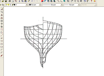
Scanned body plan image pasted into a Cad program
Now redraw the stations and the sheer line by Polylines in color red (for example). Redraw by Lines also the centerline, the design waterline and the lowest waterline. These objects will serve as frame of reference and for scaling to the full size dimensions.
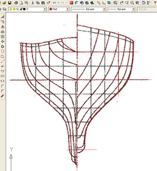
Body plan image redrawn by Polylines and Lines
Then delete the pasted picture and edit the drawing:
- Trim the stations at centerline (cl) and sheer line.
- Rotate the drawing to adjust the cl vertically.
- Draw a true horizontal design waterline (dwl); start where the redrawn one crosses cl.
- Move everything to the origin of the drawing coordinate system, using the intersection of cl and dwl as base point.
- Scale the drawing to the full size beam of the hull. The height will be corrected in MultiSurf if the initial paper lines drawing is distorted.
- Save the drawing in DXF format as body_plan.dxf.
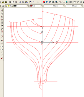
Body plan redrawn and scaled
Now repeat the procedure described above for the profile view. Just the outline is of interest, so it is less work. Save the drawing as profile_view.dxf.
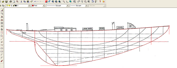
Profile view image redrawn
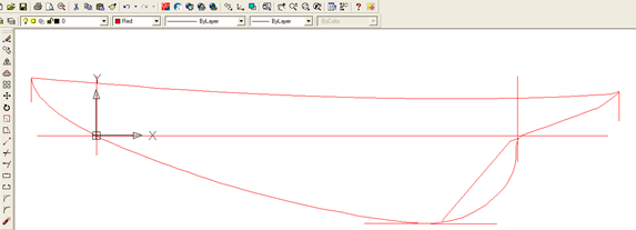
Profile view redrawn, scaled and reoriented. Station 0 at the forward end of the design waterline is at X = 0.
After these 2 steps we have transfered the body plan and profile view from the paper medium into two Cad drawings (body_plan.dxf, profile_view.dxf).
Step 3: Import DXF file into MultiSurf and save 3DA wireframe files
Regardless of how DXF files of the graphical data in the lines plan were created – with the use of some software tool or by hand - the next step is to open a new model in MultiSurf. Set the model units to those used for the Cad drawings and import the DXF files (main menu: File/ Import/ DXF). Let us continue with our file profile_view.dxf and import it into MultiSurf.
Shaded view: DXF file profile_view.dxf imported
All curves and points will lie in the XY-plane (which was the drawing plane in the Cad program). To attain the usual orientation rotate all entities around the X-axis by 90° (Edit/ Transform/ Rotate/ X-Axis).
Now it is a favourable moment to scale the heights. The draft of Dorade is given as 2.43 m. And our MultiSurf model shows, that the deepest points of the bottom of the keel is at z = -2.375 m. So Z-scale the whole model by a factor of 1.0232.
Let us look at the waterline near the bottom of the keel. Select one of the control points of the line, its Z coordinate is -1.980 m. Keep this in mind.
Profile rotated and scaled in Z to draft dimension
Before importing the DXF file of the body plan into the current model hide all entities in order to get them out of the way for the coming procedures. Then repeat the DXF import, now using the file body_plan.dxf.
DXF file body_plan.dxf imported
Again, all curves and points lie in the XY-plane. To obtain the usual orientation rotate all visible entities first around the X axis by 90°, then around the Z-axis, also by 90°.
Again check the heights in the body plan. From the profile view we know, that the waterline near the keel bottom is at Z = -1.980 m. However, the control points of the same waterline in body plan are at Z = -1.937 m. Hence we perform with all entities of the body plan a Z-scale of 1.0222.
Body plan rotated and scaled in Z to the draft dimension
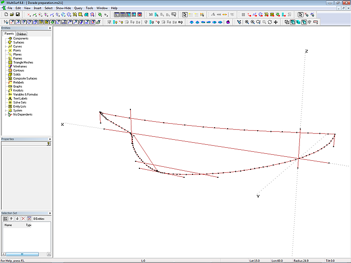
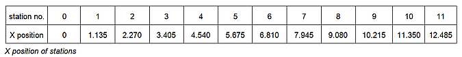
Some more operations are needed to the entities of the body plan. So far all the digitized stations lie in the YZ-plane. We must shift each station to its true X-position. Since the length of the design waterline is given as 11.35 m, equally divided in 10 intervals, the station spacing is 1.135 m.
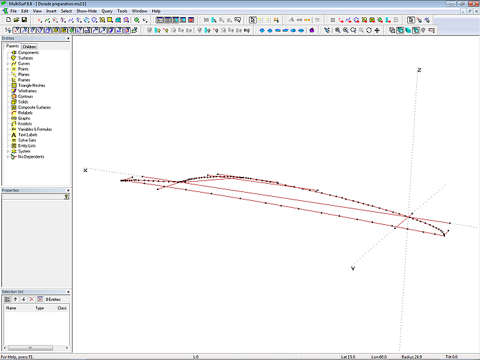
Stations shifted to corresponding X locations
Save the model as Dorade_preparation.ms2. Then select station 0 to 11 and save a 3DA wireframe file as stations.3da (main menu: File/ Export 3D/ 3DA wireframe). Next select the outline curves and save the 3DA file named profile.3da. Close the model.
Now the digitizing work using method 1 is done.
Method 2: Scale point coordinates off the drawing
A different procedure to cast the graphical data into the numerical form of a 3DA wireframe file does not need a scanner or a Cad program, but just a ruler. For each station scale a series of point coordinates off the drawing and note them down on a sheet of paper. If the drawing is given at a certain scale use the appropriate measure. If the drawing is out of scale some proportional calculations are required to obtain the point coordinates in full size.
When the measurements are finished open Windows Notepad (or any other text editor) and type in the coordinates into .3DA format.
File specification: .3DA — 3D ASCII Drawing File:
A .3DA file contains XYZ coordinates of points in ASCII format. It consists of an unlimited number of record lines each in the format:
pen x y z
pen = integer controlling pen color; 0 = pen up
x, y, z = world coordinates of point
Each line has 4 numerical entries: pen, x, y, z. ‘pen’ is the number of a color for drawing to the point (x,y,z). Each entry is separated by one or more spaces. If ‘pen’ is 0, the pen is up in moving to (x,y,z).
Example: Suppose we measured the following offsets for a station:
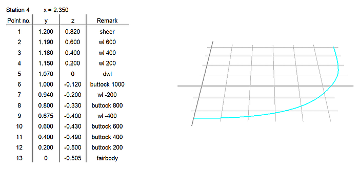
Then this lines must be typed in into Notepad and saved with the file extension .3DA:
0 2.350 1.200 0.820
7 2.350 1.190 0.600
7 2.350 1.180 0.400
7 2.350 1.150 0.200
7 2.350 1.070 0
7 2.350 1.000 -0.120
7 2.350 0.940 -0.200
7 2.350 0.800 -0.330
7 2.350 0.675 -0.400
7 2.350 0.600 -0.430
7 2.350 0.400 -0.490
7 2.350 0.200 -0.500
7 2.350 0 -0.505
Note:
- The pen value in the first line is zero, what indicates the start of the polyline.
- A 3DA file can represent more then a single curve. The begin of each curve is defined by pen = 0.
- When saving a 3DA file make sure its file extension is .3DA and not .txt or .3DA.txt.
The MultiSurf entity Wireframe displays the content of a 3DA file by a polyline passing through its points. It does not create Point entities in MultiSurf. If for some reason points are needed the command Import3DA should be used instead. This command imports a 3DA file into points and/or curves. See also the further explanations given below.
Method 3: Import Offset table
So far we discussed redrawing curves and measuring points from a lines plan on paper. Often there is also a table of offsets for the hull to be fitted. How can that one be used?
ImportTable command
MultiSurf provides the command ImportTable. It inserts a table of XYZ coordinates of points into a model.
ImportTable filename[.ext] [kind [layer]]
Imports table file into points and/or curves. If no extension is given, .TXT is used.
Kind = 0, points only
Kind = 1, Type-1 BCurves
Kind = 2, Type-3 CCurves
Let us consider an example. In the book How to build a wooden boat (David C. McIntosh, WoodenBoat Publications, Inc., Brooklin, 1987) the author presents offsets for a 39 ft sloop of his design. When this table is entered into a spreadsheet program, and feet, inches and eighths of an inch are converted to meters, we obtain the following table:
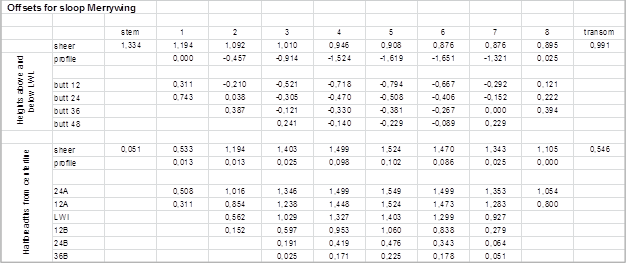
Offset table for sloop Merrywing (design: David C. McIntosh)
A table of point coordinates for use with the command ImportTable must be arranged in a specific order:
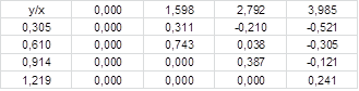
Required tabular form of input data for the command ImportTable
The string y/x in the first cell indicates, that the remaining cells of the top row hold X-coordinates, while all remaining cells of the first column hold Y-coordinates. The interior cells define the corresponding Z-coordinates. For example, the point with x = 1.598 and y = 0.610 has a z-value of 0.743. Empty cells are not allowed.
Back to the example. As first step let us import the buttock points. In the spreadsheet program add X-positions for stem, stations and transom, also y-values for the buttock locations.
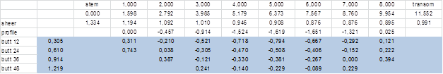
There are no entries for stem and transom so the essential table for the buttocks points will look like this:
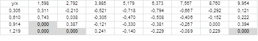
Table of buttock points for use with the ImportTable command
The grey cells indicate where zero values were entered to fill cells, for which the offset table shows no value. Select the table in the spreadsheet program, then insert its content via copy/paste into Notepad and save it as a text file (for example: butts.txt in the folder D:\temp).
Now we can import this text file into MultiSurf:
- open a new model
- use the command SetPath to specify the folder which holds the text file to process (for example: SetPath D:\temp)
- enter the command: ImportTable butts 1
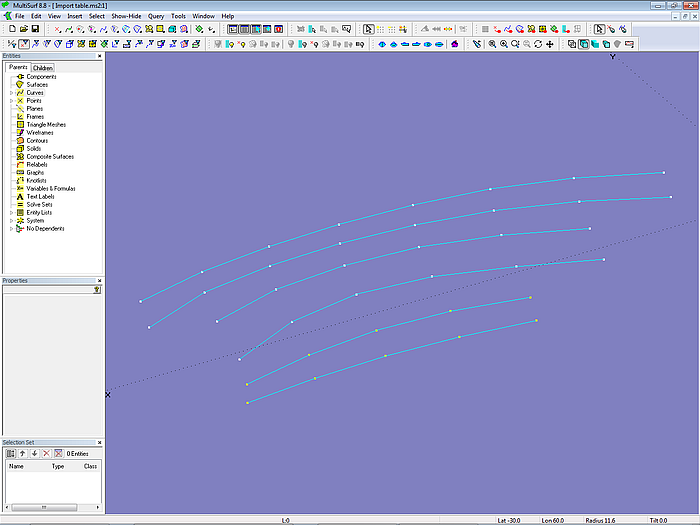
We will get the following screen image:
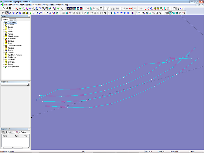
Wireframe view: buttock points imported via the command ImportTable
The screen image will look confused due to the auxiliary points. We should correct this first:
- select a curve
- in the Properties manager click in the right field of the line Control points, what will select all currently used points
- press the Ctrl key and left mouse click on those points we inserted additionally to unselect them
The screen will look much more orderly now:
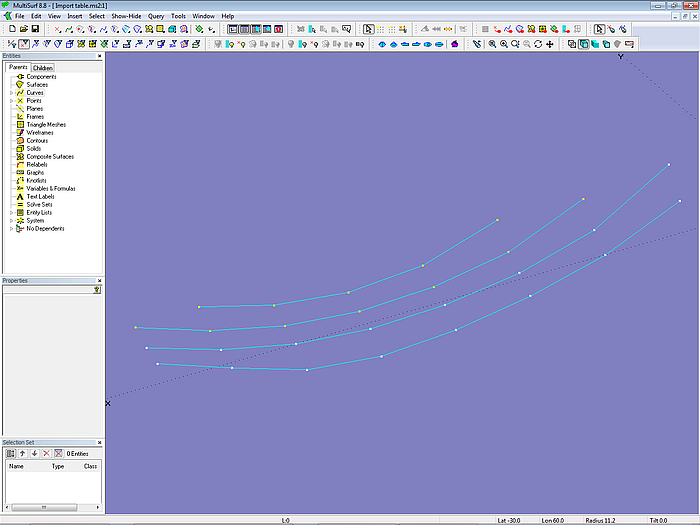
Buttocks: auxiliary points removed
The data for the waterlines are entered in the same way.
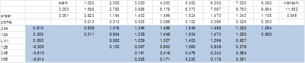
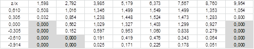
Table of waterline points for use with the ImportTable command
Again, the grey cells mark the auxiliary points to make the table complete. Save the table as wls.txt and use the command ImportTable wls 1 to insert the data.

Waterline points created via ImportTable
Again those additional zero-points should be deleted.
Waterlines: auxiliary points removed.
So far we considered points of buttocks and waterlines given in the offset table in question. These are curves with points of constant Y- or Z-coordinate values. Only this kind of point data can be inserted via the command ImportTable.
Import3DA command
In contrast to buttocks or waterlines both the Y- and Z-coordinates for points of sheer and profile vary from station to station. It is simpliest to insert their data via the command Import3DA.
Import 3DA filename[.ext] [kind [layers]]
Imports 3DA file into points and/or curves.
Kind = 0, points only
Kind = 1, Type-1 BCurves
Kind = 2, Type-3 CCurves
All what is required is to re-arrange the offsets in a differently fashioned table in the spreadsheet program and add the column for “pen”. Then save the content (marked light blue) of each table into a text file and insert those via the Import3DA command.
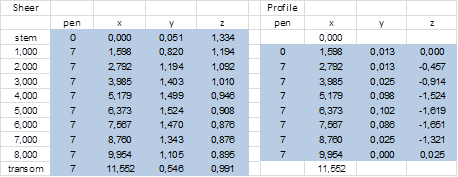
Tables for sheer points and profile points for use with the Import3DA command
Sheer and profile offsets inserted via the Import3DA command
Now show all the imported data. For each station there are points from the insertation of the waterline table and the buttock table as well as points from the import of sheer and profile. So we can finally pass through all corresponding station points a B-spline Curve of degree = 1. Before closing the model save 3DA wireframe files (File/ Export 3D/ 3DA wireframe) for the stations (mw_stations.3da) and the outline curves(mw_profile.3da).
Offset table data inserted via ImportTable and Import3DA
A table of offsets saves a lot of measuring. But since all curve data is related to the grid of the stations, the table gives no information where a curve starts and ends, or how the profile runs between stem and station 1 or beyond station 8. Thus a table of offsets must be used in combination with the lines plan drawing to complete the data input.
Pros and Cons:
None of the presented methods is superior. The accuracy of redrawing curves depends on the quality of the scan. The imported DXF data needs some transformation editing. On the other hand it is easy to digitize a curve by as many points as appropriate (not limited to the grid of the lines plan). Measuring offsets is time consuming, but the possibility to measure to the nearest grid line reduces inaccuracy which might be caused by distortion of the drawing. Including additional points between the grid lines to cover details is laborious. Importing offset table data via special commands saves time, but requires further data that has to be picked off from the drawing (bow shape, stern shape).
One should know both strengths and limits of the explained methods. Only then the best combination for the given task can be used. The surface fitting of an existing cargo vessel for CFD studies certainly requires more accurate templates than the re-design of a hull, which serves as a starting point for a related shape, which is going to be modified here and there.
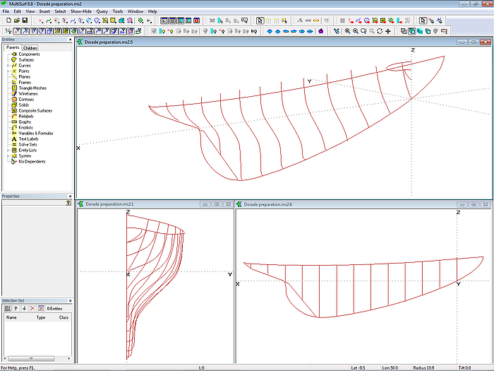
2 - Create Wireframe entities
Let us continue with the Dorade example. So far all was about the various methods to translate the existing data on paper into the numerical form of 3DA files. For Dorade we obtained those files when discussing method 1 (stations.3da, profile.3da). There the model Dorade preparation.ms2 was created. However, we will not continue with this model, but start a complete new one. Why? It was the only purpose of this model to create 3DA files for comparison purpose. Once the 3DA files exist, the model paid off its debt. If we would continue with it and start the essential fitting process therein, unnecessary ballast in form of many points and curves would be carried on.
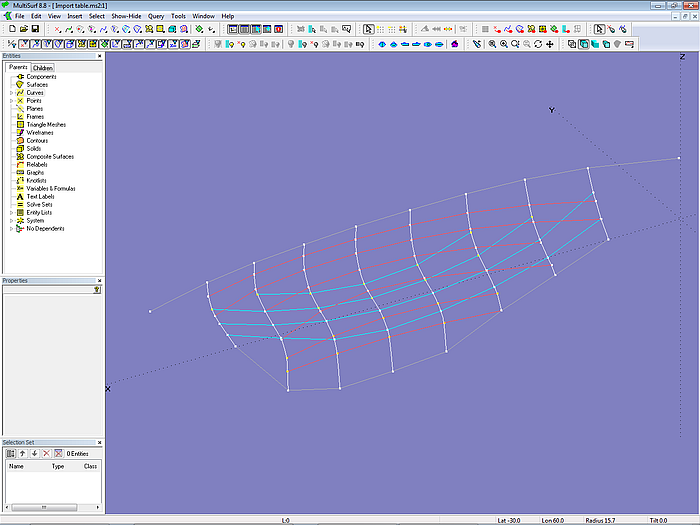
So open a new MultiSurf model and begin by creating 2 Wireframe entities from the two .3DA files stations.3da and profile.3da. The wireframe entities are the "templates", to which we will fit and compare the re-design.
Wireframe entities display the content of 3DA files.
3 - Choose surface type
The hull in question shows no rapid change of curvature in longitudinal direction, it leans to planking. Thus we decide to use a C-spline Lofted Surface, which interpolates its supporting master curves (mcs). Here the attempt is made to use a single surface for hull and keel. B-spline Curves are chosen for mcs; this type of curve is easy to bend, a complex shape needs a few control points (cps), it does not tend to oscillate.
4 - Create master curves and fill in a surface
The further procedure is basically the same as with creating a model from scratch:
- Decide about the number of B-spline mcs and their location. The first one is a portion of the stem, the last one is a little bit beyond the transom.
- Inner mcs support the surface in a regular fashion. If possibe these should lie along the digitized stations from the lines plan.
- The most complex shape determines the number of cps.
- Make mcs in a color different from the color of the wireframe.
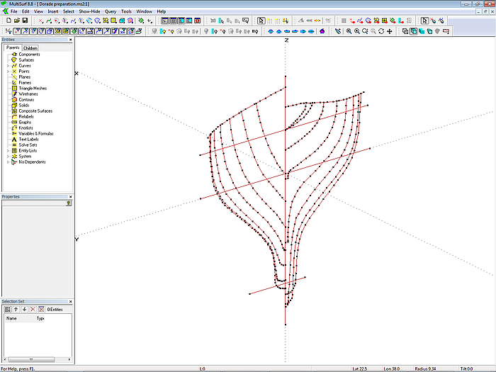
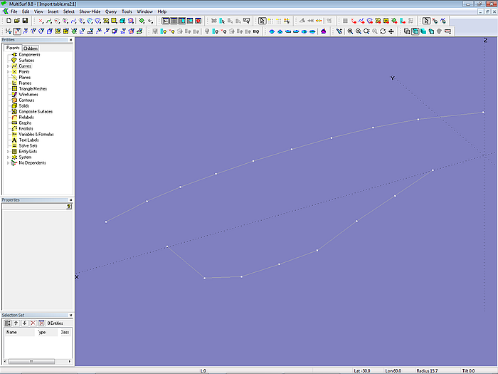
MultiSurf offers a very useful feature to create B-spline Curves from 3DA Wireframe entities: B-spline Curve Fit (main menu/ Tools/ Special). So select the stations, then do a B-spline Curve Fit; set the number of cps to 8. In a swift each station in the Wireframe entity is fitted by a B-spline Curve. Certainly some adjustment is required to improve the fitting, but B-spline Curve Fit saves much time to create the lot of cps; further, the suggested positioning of the cps along the fitted B-spline Curve is a good starting point to achieve a harmonic curvature distribution.

B-spline Curves fitted to the digitized stations
It is no good idea to use all of the generated B-spline Curves as mcs for the surface – the key to fairness is simplicity. On the other hand it is a re-design: the result should be close to the input. Thus it is a game between accuracy and fairness. Fitting can be more demanding than free-forming.
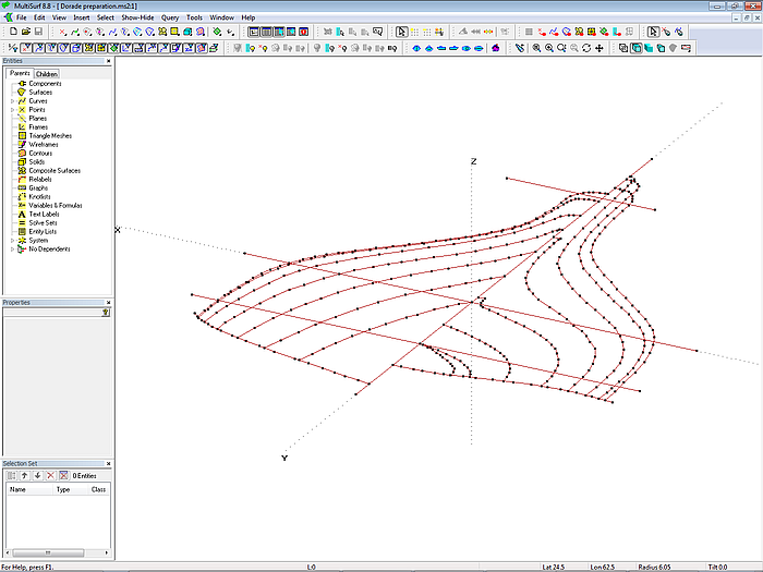
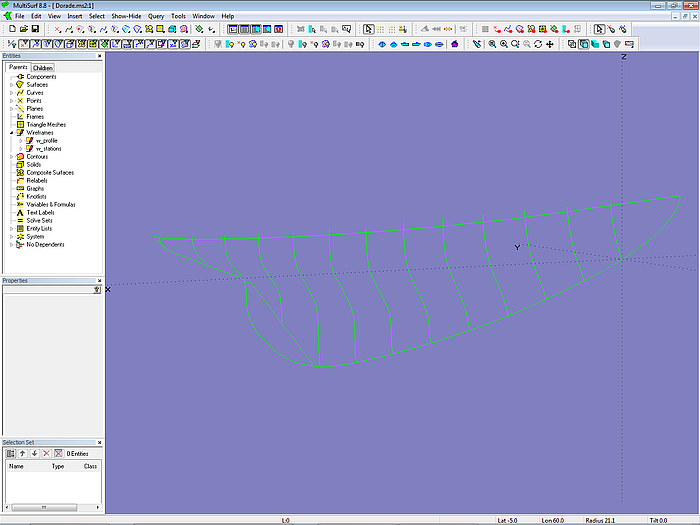
In the Dorade example every second station is used as a mc; there is a total of 10 mcs. Mc2 to mc5 run transversely, mc6 to mc8 in the aftship run sloped. Mc7 is along the slanted end of the keel. The aft mcs run partly on the negative side of the center plane to form the stern overhang.
Arrangement of mcs for the Dorade model. C-spline vertex curves are passed through corresponding cps to help fairing the surface.
5 - Check, fit and adjust
Where mcs do not lie along digitized stations make Contour entities with cuts at the same stations as represented in the wireframe data. This gives a direct comparison, and shows where we agree and where we do not. Adjustment usuallly just means going to the nearest control point on the nearest master curve and move it a little, usually normal to the surface. In general, we will have to accept some deviations from the digitized lines, because digitizing is not exact and neither was the lines plan. The one for Dorade presented in the book Yachts classiques is 15 by 7 centimeters in size.
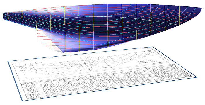
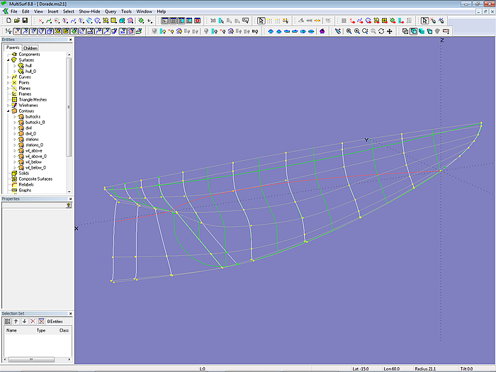
The Ship Lines view below shows the result of our efforts. There is no rudder, no transom or deck, so there is still work left. But hopefully with the help of this article it will be no problem to fit surfaces also to those given shapes.
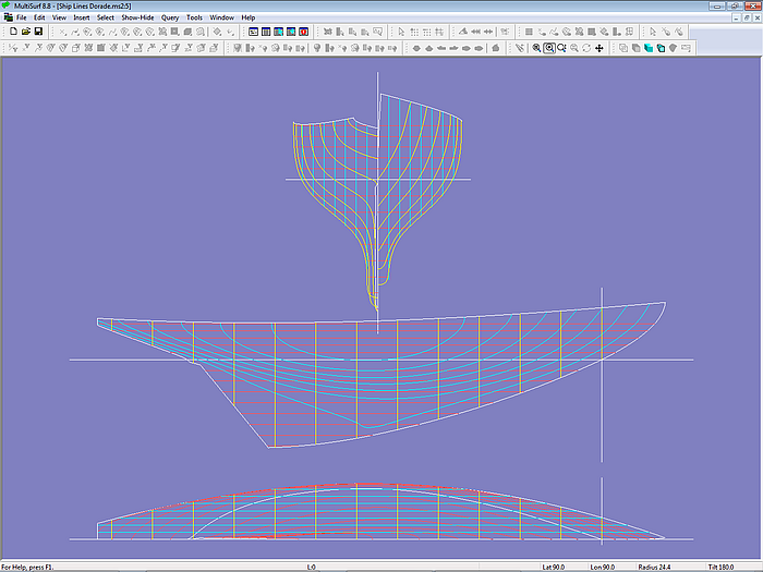
Ship Lines view of Dorade model
Further strategies for modeling traditional hulls like the one of Dorade are discussed in the separate article On the Modeling of Classic Sailing Yacht Hulls.