MultiSurf Workshop Alkmaar 2017
Selected Support Topics
compiled by Reinhard Siegel
Content:
- Modeling Moving Assemblies – Canting Keel
- How to Model a Sheer Clamp
- Frame as Mirror
- Similar Label
- Command WriteOfe
Modeling Moving Assemblies
Model canting_keel.ms2
To move in a model a part of the geometry relative to the overall geometry all its control points must be related to its own frame of reference. If the position of this coordinate system is changed in space, all its dependent objects will change with it. The model canting_keel.ms2 shows an example.
F0 is a Roll-Pitch-Yaw Frame (RPY Frame). Its origin is determined by Point ip_keel, the value for the property Roll defines the rotation about its X-axis.
All control points of the keel-fin surface and the keel-bulb surface are based on this frame F0. If the value for Roll is changed, the inclination of the keel will change too.
The model is not symmetrical to the centerplane (XZ-plane of the global coordinate system) at model level. That is why the hull surface and rudder surface are reflected with regard to the centerplane by Mirrored Surfaces. Also the port side of the fin surface is a Mirrored Surface, but here the mirror plane is the 2 Pt Plane a0. It is perpendicular to the Y-axis of the RPY Frame F0. The ballast bulb is a Revolution Surface, the meridian curve is the Foil Curve c11; the angle of rotation is 360°, so port and starboard side are in one.

Model canting_keel.ms2
How to Model a Sheer Clamp
Model sheer_clamp.ms2
Model sheer_clamp.ms2 explains how to construct the sheer clamp of a wooden boat. The cross-section of the clamp should be rectangular and it should be fastened to the hull area in such a manner, that at any section the upper corner point lies on the sheer edge, while the lower corner touches the hull surface.

Model sheer_clamp.ms2
The EdgeSnake ue_hull runs along the top edge of the hull. On this snake the Ring ring1 is located. Depending on the ring is the Tangent Point pt1, its offset value determines the height of the clamp´s cross section (here 6 cm). Also child of ring1 is the Offset Point pt2. Between pt1 and pt2 the Line line1 is set up.
Now pt1 is rotated around this line by 90 degrees - result is the Rotated Point pt3.

Tangent Point pt1 and Offset Point pt2 are children of Ring ring1 on the EdgeSnake ue_hull. Point pt1 is rotated around Line line1 by 90 degrees yielding Rotated Point pt3.
Since, in general, the hull surface is curved in transverse direction, pt3 will not rest exactly on the hull surface. That is why pt3 is to be projected onto the hull surface, which results in the Projected Magnet m1.
With Ring ring1, Projected Magnet m1 and the Tangent Point pt1 the 3-point Frame frame1 is produced.

3-point Frame frame1, defined by Ring ring1, Projected Magmet m1 and Tangent Point pt1
Based on this frame, the Point pt4 is created - its dz value is the thickness of the clamp (here 2 cm). The point pt5 is a Copy Point, which makes safe that the points ring1, m1, pt4 and pt5 are at right angles to each other and lie in a common plane. The B-spline Curve curve1 (degree = 1) is connecting these points.

Cross section of the clamp at the location of ring1
Thus, the cross section of the clamp at the location of ring1 is now determined. Finally its construction is repeated for all positions of ring1 by the the Procedural Surface sheer_clamp. Its moving curve is curve1, the driving point is Ring ring1.
Frame as Mirror
Model frame_as_mirror.ms2
MultiSurf offers as secondary coordinate systems the entities 3-point Frame and RPYFrame. Apart from its function as arbitrarily positionable frame of reference, a Frame can also be used where an entity definition requires to specify a Mirror/Surface object. Examples are Contours, Intersection Beads/ Rings/ Snakes or Mirrored Points/ Curves/ Surfaces. The plane spanned between X- and Y-axis of the frame then serves as mirror object.
Model frame_as_mirror.ms2 shows this additional function of the Frame entities.

Model frame_as_mirror.ms2 - if a frame is specified as a Mirror/ Surface object, its XY plane serves as a mirror.
In the example, the 3-point Frame F0, determined by the points pt1, pt2 and pt3, is specified in the definition of the Contour dwl_0. Likewise for the Mirrored Point pt5.
Similar Label
Quotation from MultiSurf Help:
All of the curves you can form in MultiSurf are defined by reference to a “parameter” t, which takes the value 0 at one end of the curve (the “start”) and 1 at the other end (the “end”). The rule that defines the curve from its data points is written, mathematically or in computer code, in terms of the variation of t. You can think of each point of a curve as being labeled by a specific value of t (Fig. 1). In many situations t is roughly the arc length from the start of the curve to a given point, divided by the total arc length between the curve ends.

Fig. 1 A curve marked at t = .1 intervals
It is quite accurate and appropriate to think of the generation of a parametric curve as being a continuous mapping or correspondence between the real numbers from 0 to 1 and points in 3-dimensional space (Fig. 2). You can also think of the curve as being the path of a moving point and t as being time.

Fig. 2 A representation of the t parameter space corresponding to Fig. 1
Why this preface? Its purpose is to better understand what labeling and relabeling is all about. And how one can make the labeling of a curve similar to another curve. Let us consider this topic in the following example model relabel-1.ms2.
The model includes the topside surface of a workboat, the bowround and a bulwark. The bulwark is a Ruled Surface, spanned between the B-spline Curve c2 and the PolyCurve c1, a combination of the top edge of the bowround surface and a portion of the sheerline.
A Ruled Surface is created from two curves by connecting points on each parent curve having equal t parameter values with straight lines (the “rulings”).

Model relabel-1.ms2 - bulwark as Ruled Surface spanned between B-spline Curve c2 (top edge) and PolyCurve c1 (bottom edge)
The station contours of the bulwark are hollow at the end of the bow. The reason for this is the strongly inclined run of the rulings. On curve c1 the ruling endpoints lie farther aft than the corresponding end points on the bulwark top edge (curve c2).
If the bulwark stations are to be straight, the rulings must run vertically. In order to achieve this, the the t-parameter distribution of either of the two parent curves of the Ruled Surface has to be changed (relabled).
There are several entity options for this:
- Relabel
- SubCurve
- Procedural Curve
Relabel Entity
As a result of their mathematical definition curves, snakes and surfaces own an inherent "natural" distribution of the t-parameter, the default labeling. This is in effect when the default "*" is used for the Relabel property. If instead a Relabel entity is specified, then this one will determine the parameter distribution.
For further details of the Relabel entity please refer to the user documentation or the program Help.
SubCurve
A clear method and intuitively to use is the control of the parameter distribution offered by the curve type SubCurve. Usually two beads are used to define a section of a curve, one at the beginning, one at the end of the section. But if some more beads are placed between these two, the parameter distribution can be manipulated visually.
Model relabel-2.ms2 illustrates this approach for our example.

Model relabel-2.ms2 – here the parent curve at the bulward top is SubCurve c3. Moving inner beads modifies its t- parameter distribution.
Three beads, e1, e2 and e3, are based on the B-spline Curve c2 (bulwark top edge). With these and the system beads *0 (t = 0) and *1 (t = 1) the SubCurve c3 is defined. Parent of bulwark surface is now c3 instead of c2. Moving the beads will change the distribution of the t-parameter along curve c3, thus the run of the rulings of the Ruled Surface changes what finally effects the cross section shape of the bulwark.
Procedural Curve
With the help of a calculation formula one can also create a procedural curve whose labeling is similar to another curve. Model similar_label.ms2 shows the principle.
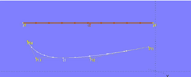
Model similar_label.ms2 – tickmarks illustrate the different labeling of curves c1 (B-spline) and c2 (Line).
The model holds the B-spline Curve c1 and the curve c2 (here a Line entity). The tickmarks (curve point at t = 0.1, 0.2, 0.3, etc.) clearly show the different labeling of both curves. The task is now to relabel curve c2 so that on both curves for the same t-parameter the ratio of arc-length distance (length measured along the curve from its start to the curve point) to total curve length is equal. Of course, the shape of the curve c2 must remain unchanged by the relabeling.
For this purpose, the bead e1 is set on curve c1. The arc-length distance from t = 0 to e1 can be calculate by the formula
arcdist_c1 = ARCLEN (c1, 0, TPOS (e1))
The total length of c1 is:
length_c1 = ARCLEN (c1, 0, 1)
The ratio of both lengths is x:
arcdist_c1 / length_c1 = x
Now the arc-length distance on curve c2 is looked for, which results in the same ratio.
The total length of c2 is:
length_c2 = ARCLEN (c2, 0, 1)
Let arcdist_c2 be the wanted arc-length distance. Then it applies:
arcdist_c2 / length_c2 = x
Replacing x:
arcdist_c2 / length_2 = arcdist_c1 / length_1
or
arcdist_c2 = arcdist_c1 * (length_2 / length_1)
Finally, with the formulas stated above:
arcdist_c2 = ARCLEN (c1, 0, TPOS (e1)) * (ARCLEN (c2, 0, 1) / ARCLEN (c1, 0, 1))
That is, for point e1 on curve c1 a corresponding point on curve c2 is looked for, which is located the arc-length distance equal to the value arcdist_c2 measured along c2 from t = 0. This is the Arc length Bead e2 with arc dist = arcdist_c2.
To repeat this construction of e2 for all possible positions of e1 on curve c1, the Procedural Curve c3 is created. Its moving point is e2, the driving point is e1. Each point on curve c1 with the parameter value t now corresponds to a point on curve c3 with the same parameter value t, and for both curves the ratio of arc-length distance to total length is the same. Thus, curve c3 has the same labeling as curve c1.

Model similar_label.ms2 – Procedural Curve c3 relabels Line c2 similar to the B-spline Curve c1.
In the model relabel-3.ms2 this method is used to relabel the upper parent curve of the bulwark.

Model relabel-3.ms2 - the Procedural Curve c3 along the bulwark top edge got the same labeling as the curve c1 along the lower edge.
Command WriteOfe
Suppose we want to calculate the hydrostatics of a ship hull. There is a linesplan on paper and even a DXF file of cross sections. Those are B-spline Curves degree = 1 and their number would be sufficient for the required accuracy, so fitting a surface to the lines can be saved.
How can we make an OFE file for Hydro from the DXF file?
1 Import DXF
First import the DXF file via File/ Import/ DXF into MultiSurf. This is the model import-1.ms2.

Model import-1.ms2 - DXF file of the transverse cross sections imported (B-spline Curves, degree =1)
2 OFE file specification
- Only one half of a station is represented. (Bilateral symmetry is assumed in an .OFE file).
- First and last point in a station must have Y = 0.
- Points go around half-station counterclockwise when viewed from astern: beginning at the base of the keel and continuing up the starboard side of the hull, across the deck, etc., and back to centerline.
As can be seen, the imported stations are not closed and their orientation is downwards from the deck side.
3 Change orientation
To change orientation, select a curve for display in the Properties manager, then click in the right part of the property "Control points", which causes the Selection Set to list all is parent points. In the Selection Set now click the command button "Reverse order of set" - the order is changed. Finally, confirm with "Ok" in the Properties manager.

Command button” Reverse order of set” in the Selection Set manager
Repeat these steps for all stations. This is model import-2.ms2.

Model import-2.ms2 – cross sections with ascending orientation of control points
4 Close stations
The stations in an OFE file must be closed, that is, each curve must start and end on the centerplane. Although the stations in our the example all begin on the centerplane, but they end up on the side of the hull.
Further, if a station is made up by several portions, as it is the case here at the bulbous bow and at the stern, it must be combined into a single curve.
In order to extend the stations to the centerplane, all the first points on the side of the hull are projected onto the centerplane as Projected Points. The function "Create Copies" is very useful here (main menu/ Insert/ Copies or key "c"). First choose the entity to be copied, here the first Projected Point, then all the remaining points that should also be projected. Click on "Ok" and all Projected Points are on the screen.
Then select each station curve for edit: add the corresponding point on centerplane to its list of control points.

Model import-3.ms2 – all stations start and end on the centerplane; piece-wise defined station are joined together.
In our example, the first two stations at the bow and the second but last station at the stern are defined in two parts. As for an OFE file a continuous curve required, they must be assembled. A PolyCurve can not be used for this. The control points of one piece must be added to the control points of the other one. This is model import-2.ms2.
5 Save OFE file – command WriteOFE
After this preliminary work to ensure that the data is in the proper format the OFE file is saved using the command "WriteOFE". Commands are entered in the dialog box “Command Window” which is accessed via main menu/ Tools/ Command Window.
However, first the storage location must be specified. This is done by the Command "SetPath". In the example here the file path is to be: D:\Temp.

Command SetPath

Command WriteOFE
The easiest way to choose all stations for export is to drag a selection window from top left to bottom right. Then main menu/ Tools/ Command Window (or key "w") to open the dialog box. In the command line, enter "WriteOFE" and the file name.

Command WriteOFE

Command WriteOFE
6 Check – import OFE file
To check whether everything was done properly one can import the saved OFE file with the command "ImportOFE". Just open a new model and enter in the command line: ImportOFE test99.
The commands WriteOFE and ImportOFE add to MultiSurf the functionality of an offset file editor.
By the way, all commands available via the Command Window are listed using the command "Help".

List of Commands
======================================================================================