About Hull Shapes with Vanishing Chine
Two methods
by Reinhard Siegel
March 2024
Content
Introduction
1 Hull with vanishing chine – the Two-Surface approach
1.1 Master curves connected tangentially
1.2 Master curves split into SubCurves
2 Hull with vanishing chine – the One-Surface approach
3 Examples
3.1 Sailing ship hull – rounded stern with vanishing chine
3.2 Powerboat hull – foreship with vanishing chine
4 Summary
5 Appendix – The Vertex Curve Method
Introduction
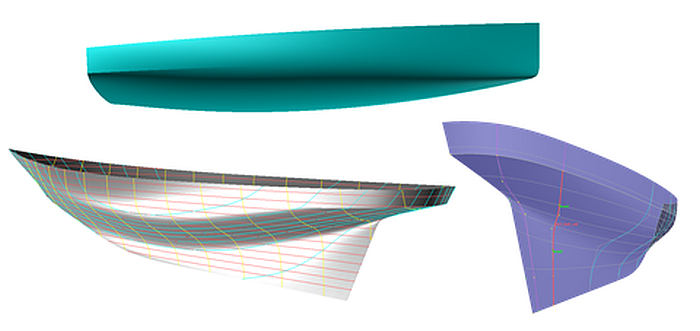
The shape of ship and boat hulls is diverse. Stations, i.e. cross-sections through the hull surface, harmoniously change their shape from bow to stern. For their part, stations themselves can have an unsteady shape. For example, if the stations in the forebody shows much flare, a break in the section curve can prevent the deck from becoming excessively wide. The same applies to sailboat hulls, here in the stern area. If these station break points are connected, a chine curve is created that runs in the longitudinal direction of the hull. Depending on the type of boat, the chine can run relatively close to the upper edge of the hull or be significantly lower in the section girth dimension.
A chine curve can extend the entire length of the hull from bow to stern. Then the discontinuity in the station gradually changes in the longitudinal direction, but does not disappear completely.
However, a chine curve can only occur in a certain hull area. Then the discontinuity gradually disappears and the stations run smoothly.
Modeling a hull with a full length chine is easier than modeling a hull with a partial length chine. In Tutorial 2, Round Bilge Hull With Full Length Chine, the former design issue is discussed. In Tutorial 3, Round Bilge Hull With Vanishing Chine, a method is presented on how a hull with a partial length chine in the stern can be created (in Tutorial 22, Three Modeling Exercises, the method shown is used for a catamaran hull).
This tutorial here discusses further methods of how to model various hull shapes with a vanishing chine.
Abbreviations used:
cp: control point (support point)
mc: master curve = support curve
cp1, cp2, ...: denotes 1st, 2nd, ... point in the list of supports of a curve. It is not an actual entity name.
mc1, mc2, ...: denotes 1st, 2nd, ... curve in the list of supports of a surface. It is not an actual entity name.
In the following the terms used for point, curve and surface types are those of MultiSurf. This may serve the understanding and traceability.
1 Hull with vanishing chine – the Two-Surface approach
In the Two-Surface approach, the chine curve is extended to run the entire length of the hull. It also runs in an area where the stations have no break point but are of smooth shape.
Along the chine, the hull is divided into an upper surface and a lower surface. There are two ways to create these two surfaces:
- Connect master curves tangentially
- Split master curves into SubCurves
1.1 Master curves connected tangentially
Since this method is already described in Tutorial 3, the essential procedure will be briefly summarized using the model sailboat-tangent_mcs.ms2 as an example. Both surfaces are C-spline Lofted Surfaces (topside, bottom), supported by the same number of master curves (mcs). All mcs are B-spline Curves with the same degree. All mcs of a surface have the same number of control points (cps). The last cp of a side master curve is also the first cp of the corresponding bottom master curve. So the mcs for side and bottom are separate B-spline curves, but touch each other.
In the aft part of the hull, where the stations should show a break point, the pairs of master curves for side and bottom meet with different tangent direction. In the front fuselage area, where the stations should run smoothly, the mcs join up tangentially.
Unlike in Tutorial 3, in model sailboat-tangent_mcs.ms2 the entity Tangent Point is used for the tangential joint. For this purpose, on each of the front mcs for the surface bottom a Bead is inserted at the start of the curve (t = 0); on this Bead a Tangent Point depends. The mcs of topside are defined with cp1 and these two points. The Tangent Point hardwires the tangential connection of the mcs of the top and bottom surfaces.
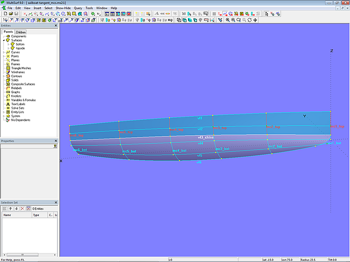
Model sailboat-tangent_mcs.ms2 – 6 mcs each support the C-spline Lofted Surfaces topside and bottom. In the smooth part of the hull the mcs for side and bottom join each other tangentially. Vertex curves pass through corresponding control points.
Advantage:
When constructing the model in this way, the vertex curve method can be used for fairing (see appendix). The chine is also a vertex curve (C-spline Curve vl3_chine). Its run is directly determined by the corresponding cps.
Disadvantage:
In the smooth part of the hull (stations without break point), the mcs for side and bottom touch with continuous tangent direction, but the curvature can be discontinuous. To control the curvature, one can assemble a corresponding pair of mcs by a PolyCurve entity and then check its curvature profile via View/ Display/ Profile/ Curvature (or toolbar button).
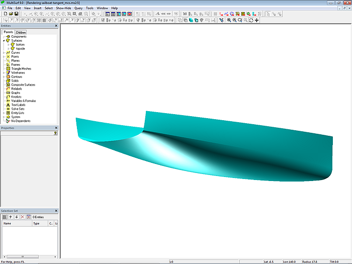
Model sailboat-tangent_mcs.ms2 – vanishing stern chine
1.2 Master curves split into SubCurves
Wouldn't it also be possible to use in the smooth part of the hull continuous mcs from the top to the bottom edge, but then divide these into 2 SubCurves each? Then the mcs for side and bottom will meet with both same tangent direction and same curvature. This is tried out in model sailboat-subcurve_mcs-0.ms2.
Base hull
A hull with a partial length chine is not too far from a smooth hull. The area with continuous stations is larger than the area with breaks. That is why it makes sense to start by modeling a smooth hull that has the desired shape except for the vanishing chine. The vertex curve method can be used for fairing so that corresponding cps change their position harmoniously in the longitudinal direction of the hull surface and thereby also make the u-parameter curves run fair. The mcs then will have a similar parameter distribution among themselves, which they pass on to SubCurves. For more information about the vertex curve method, see the appendix.
The base surface is the C-spline Lofted Surface hull_fair, defined with 6 B-spline mcs and 6 cps each. The vertex curve method with the C-spline Curves vl1 to vl6 is used to support fairing.
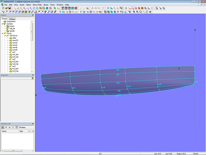
Model sailboat-subcurve_mcs-0.ms2 – the C-spline Lofted Surface hull_fair without chine is supported by 6 mcs. Corresponding control points are connected by vertex curves as a fairing aid.
If the vertex curves run regular, the u-parameter curves (lofting curves) and thus the lofted surface is smooth.
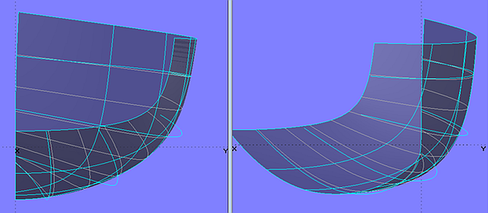
Model sailboat-subcurve_mcs-0.ms2 – vertex curves and u-parameter curves (lofting curves) of the C-spline Lofted Surface hull_fair
Split forward master curves
The forward mcs of the base surface are now divided to create the mcs for the side and bottom surfaces in the smooth part of the hull. One Bead (e1 to e4) is placed on each of the 4 front mcs (mc1 to mc4) and the SubCurves mc1_top, mc1_bot, mc2_top, mc2_bot etc. are determined with these. With the Beads and the two free Points p53_a and p63_a at the X-position of mc5 and mc6, the C-spline Curve chine is then defined. In contrast to model sailboat-tangent_mcs.ms2, the curve chine no longer corresponds to the vertex curve vl3.
The rear mcs in the hull area with chine (mc5_top, mc5_bot as well as mc6_top and mc6_bot), which “bulge” the hull surface outwards and downwards, are taken from the model sailboat-tangent_mcs.ms2.
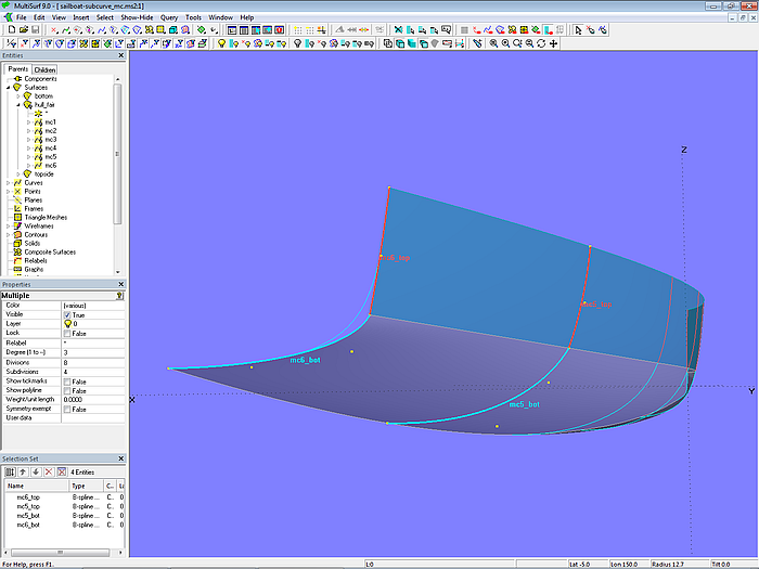
Model sailboat-subcurve_mcs-0.ms2 – the surfaces topside and bottom are supported in the stern area by the B-spline mcs mc5_top, mc5_bot, mc6_top and mc6_bot; they meet with a break.
After this preparatory work, the C-spline Lofted Surfaces topside and bottom can now be created analogous to the model sailboat-tangent_mcs.ms2.
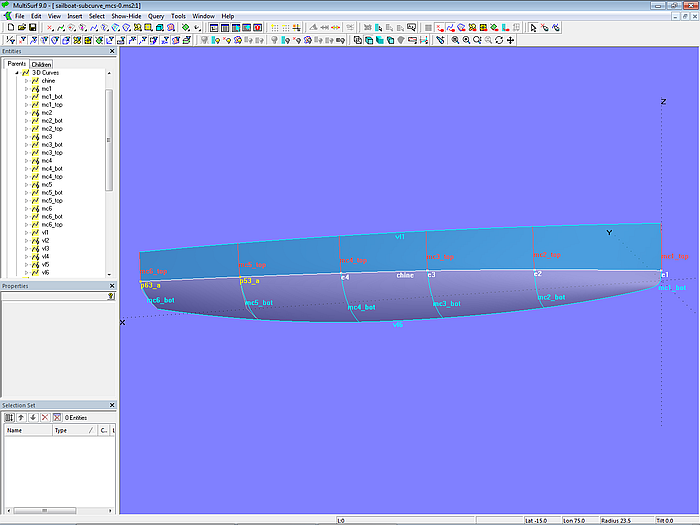
Model sailboat-subcurve_mcs-0.ms2 – master curves of the C-spline Lofted Surfaces topside and bottom.
Run of the u-parameter curves
In order to check the fairness of the two surfaces topside and bottom, let us look at the run of their u-parameter curves. It can be seen that their shape is not harmonious for bottom. The reason for this is the difference in the parameter distribution of the rear mcs (B-spline Curves) to the parameter distribution of the front mcs (SubCurves). The parameter distribution of the front mcs is similar, as it is inherited from the continuous mcs of hull_fair to the SubCurves.
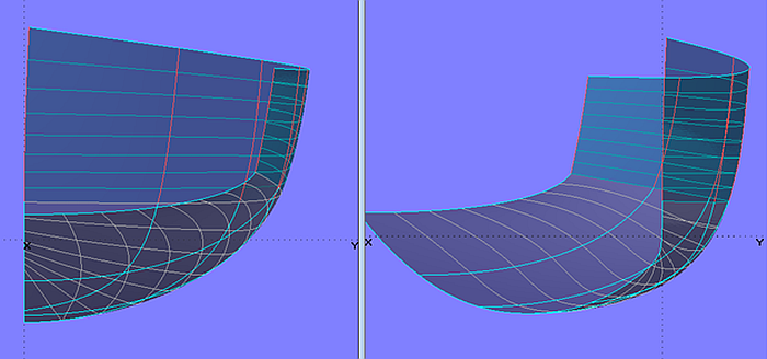
Model sailboat-subcurve_mcs-0.ms2 – u-parameter curves (lofting curves) of the C-Spline Lofted Surfaces topside and bottom. Due to the different parameter distribution of the aftbody mcs, the u-parameter curves are not regular.
When building such a hull in practice, one will move the planks or strips along the rear mold frames slightly until there run looks nice and sweet.
Option 1: relabel rear mcs with SubCurve
Applied to our model, this means that the curve points of the two B-spline Curves mc5_bot and mc6_bot must be assigned other t-parameter values (re-parameterization, relabel). The shape of the curve does not change when relabeling, the position of the curve points also remains the same, only the associated t-parameter value is changed. The easiest way to relabel a curve, because it is very clear, is to use the SubCurve entity.
Since we know from surface hull_fair that its mcs have a regular arrangement of their cps in the longitudinal direction, and consequently also a regular parameter distribution, it is obvious not to change these mcs, but only to relabel the mcs in the aftbody. This is demonstrated in model sailboat-subcurve_mcs-1.ms2.
First the Bead bead1 is put on mc5_bot and the Bead bead2 on mc6_bot. Then the SubCurve mc5_bot_sub is created with the control beads {*0 bead1 *1} and the SubCurve mc6_bot_sub with {*0 bead2 *1}. Finally, in the definition of the surface bottom these two SubCurves are used instead of mc5_bot and mc6_bot.
If now the Beads bead1 and bead2 are moved, the u-parameter curves also shift. When viewed from different directions these run harmoniously, the surface is fair.
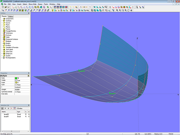
Model sailboat-subcurve_mcs-1.ms2 – mc5_bot and mc6_bot relabeled with SubCurves. By moving the Beads bead1 and bead2, the shape of the u-parameter curves is modified.
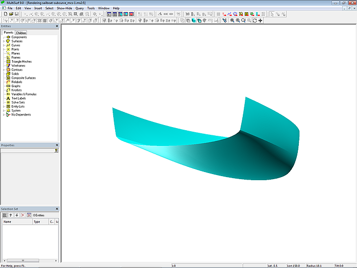
Model sailboat-subcurve_mcs-1.ms2
Option 2: rear mcs with additional control point
Instead of relabeling the rear mcs mc5_bot and mc6_bot using SubCurves, these two B-spline Curves can alternatively be defined with an additional control point each. This way will gain a little more freedom – one can give the curves the desired shape and at the same time influence the run of the lofting curves.
This procedure is shown in model sailboat-subcurve_mcs-2.ms2. Mc5_bot and mc6_bot now have 5 cps instead of 4 cps. Their inner cps are positioned so that the curves have the same shape as the mcs in the models already presented, but at the same time a regular course of the u-parameter curves results.
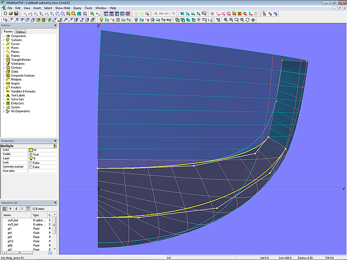
Model sailboat-subcurve_mcs-2.ms2 – B-spline Curves mc5_bot and mc6_bot defined with additional control point
Advantage:
The vertex curve method can be used to create the smooth base hull (hull_fair). The mcs for the smooth part of the hull are formed as a whole, not separated. They are continuous in direction and curvature. The parameter distribution of the mcs is similar. The chine can be changed without having to change the shape of the master curves at the same time.
Disadvantage:
Because one first has to model a smooth base hull (hull_fair) the effort is slightly greater than with the separate mcs approach (model sailboat-tangent_mcs.ms2). The vertex curve method can be used for hull_fair. However, since there are no corresponding cps on the front mcs, such guiding curves cannot be generated for positioning the inner cps of the rear B-spline Mcs (mc5_top, mc5_bot, mc6_top, mc6_bot). That is why when arranging the cps for these mcs, in addition to the desired shape, one also has to keep an eye on the harmonic run of the u-parameter curves (lofting curves) of the C-spline Lofted Surfaces topside and bottom. By SubCurve relabeling or with additional cps one must modify the parameter distribution of the mcs in the hull area with chine.
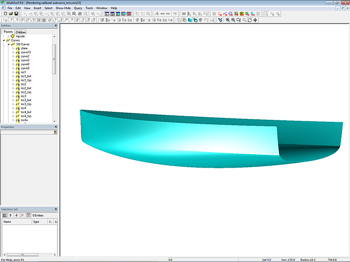
Model sailboat-subcurve_mcs-2.ms2
2 Hull with vanishing chine – the One-Surface approach
In the so far presented models sailboat-tangent_mcs.ms2 and sailboat-subcurve_mcs.ms2 the hull is split into two surfaces along the chine curve: a side surface and a bottom surface are supported by separate mcs. However, the One-Surface approach only uses mcs that run from the top edge to the bottom edge of the hull. For the rear mcs that have a break point the entity PolyCurve is used. With this type of curve, the curve segments for hull side and hull bottom are combined into one curve.
Starting from model sailboat-subcurve_mcs-0.ms2, the One-Surface approach is shown in model sailboat-polycurve_mcs-0.ms2. The SubCurves (mc1_top, mc1_bot etc.) on the forward mcs are no longer necessary. The B-spline Curves mc5_top and mc5_bot as well as mc6_top and mc6_bot are combined to the PolyCurves mc5_poly and mc6_poly.
A note about the PolyCurve entity – there are two variants of the PolyCurve, determined by the “Yes/No” entry in the “Specify end t-values” line in the Properties Manager. The default is “No”. The curve is then created so that the curve points are evenly distributed along the length of the curve. If the respective t-parameter value is to be specified at the end of the individual PolyCurve segments, “Yes” must be selected.
We set “Specify end t-values” to “Yes” and as a test give both PolyCurve mcs the value 0.220 for the end of the segments mc5_top and mc6_top.
The final surface with partial length chine can now be created with the B-spline mcs mc1 to mc4 as well as the two PolyCurves mc5_poly and mc6_poly (C-spline Lofted Surface hull_w_chine).
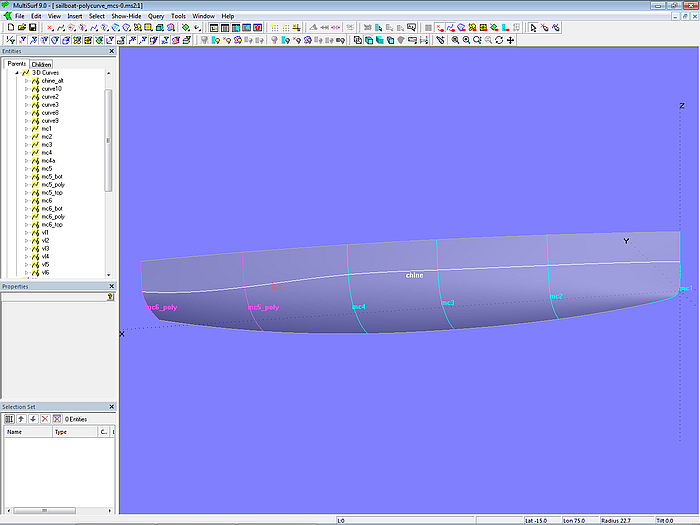
Model sailboat-polycurve_mc-0s.ms2 – C-spline Lofted Surface hull_w_chine with continuous B-spline mcs at the front and PolyCurves at the rear. End t-value of the PolyCurve-mcs set to 0.220 as a test.
In the Two-Surface approach the chine curve is equivalent to the EdgeSnake along the lower edge of the surface topside or along the upper edge of the surface bottom. In contrast, in the One-Surface approach the chine is a UVSnake in the u-direction, defined with a magnet whose u-value is equal to the end t-value of the PolyCurve-mcs. So the chine curve is a very specific u-parameter curve.
To create the UVSnake chine for the surface hull_w_chine, we place the Magnet m_chine on the surface and select for its u-value the end t-value, which is used for the PolyCurves mc5_poly and mc6_poly.
The end t-value for mc5_poly and mc6_poly must be chosen appropriately so that the UVSnake chine is fair. At the value of 0.220 used as a test, chine does not run harmoniously. The curve point at the front mcs, which belongs to this t-parameter value, is closer to the start of the curve than at the rear mcs.
Since nothing should be changed on the front mcs - the u-parameter curves of the base surface hull_fair are smooth – one has to find the appropriate value by trial and error. With an end t-value of 0.296 for the PolyCurves (magnet m_chine with the same u-value), the UVSnake chine runs regularly.

Model sailboat-polycurve_mc-0s.ms2 – C-spline Lofted Surface hull_w_chine with continuous B-spline-Mcs at the front and PolyCurve-mcs in the rear area. End t-value set to 0.296.
Let's now look at the shape of the u-parameter curves of model sailboat-polycurve_mcs-0.ms2.
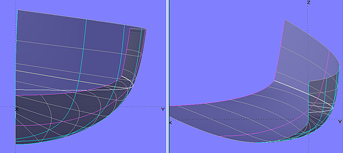
Model sailboat-polycurve_mcs-0.ms2 – u-parameter curves of the C-spline Lofted Surface hull_w_chine (continuous B-spline mcs in the front and PolyCurves aft)
As in the model sailboat-subcurve_mcs-0.ms2, the lofting curves below the chine are not regular. The cause is the same - the different parameter distribution of the rear mcs compared to the parameterization of the front mcs. Since we know from the surface hull_fair that these mcs have a regular arrangement of their cps in the longitudinal direction, and consequently also a regular parameter distribution, it is obvious not to change these mcs, but only the mcs positioned in the aftship.
As with the Two-Surface approach, two options are available. On the one hand, one can relabel the rear mcs mc5_bot and mc6_bot with SubCurves and use them as a PolyCurve segment. This is shown in model sailboat-polycurve_mcs-1.ms2.
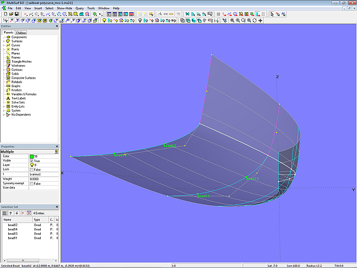
Model sailboat-polycurve_mcs-1.ms2 – mc5_bot and mc6_bot relabeled with SubCurves. By moving the Beads bead1 and bead2 the run of the u-parameter curves can be modified.
On the other hand, one can define mc5_bot and mc6_bot with additional cps. Model sailboat-polycurve_mcs-2.ms2 uses one more cps.
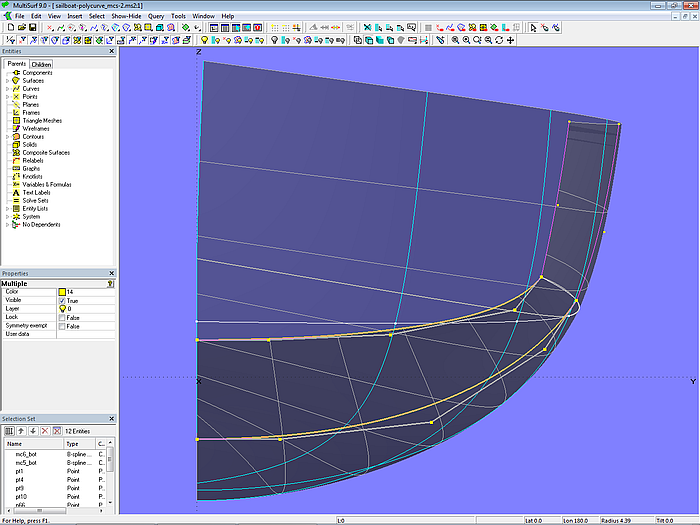
Model sailboat-polycurve_mcs-2.ms2 – B-spline Curves mc5_bot and mc6_bot defined with additional control point
Advantage:
The vertex curve method can be used for the smooth base hull (hull_fair). The mcs in the smooth hull area are formed as a whole, not separated. They are continuous in direction and curvature. The parameter distribution of the mcs is similar. The chine curve can be easily changed without simultaneously changing the Mc shape. Lower number of objects = less effort.
Disadvantage:
The chine curve depends on the “end t-values” of the PolyCurves. One has to choose the value so that the final surface shows a fair u-parameter curve. That means trial work. If necessary, the PolyCurves must be re-parameterized in order to obtain smooth u-parameter curves.
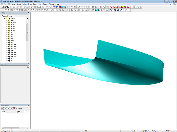
Model sailboat-polycurve_mcs-2.ms2
3 Examples
The hull shape of sailing ships (clipper, fast cargo sailor, classic yacht) often shows two distinctive features - a rounded stern with a chine in longitudinal direction. Another example is the hull of a powerboat. In order to limit the flare of stations, the otherwise round-bilge hull has a partial length chine in the foreship.
3.1 Sailing ship hull – rounded stern with vanishing chine
Taking the hull shape of a yacht as an example, we will show how this geometry can be modeled using the Two-Surface approach and the One-Surface approach.

Classic yacht – rounded stern with partial length chine
3.1.1 Two-Surface approach – master curves tangentially connected
As described in Section 1, this approach extends the chine to the bow, creating a longitudinal curve that divides the hull into two surfaces. On some ships the side deck curve is the extension of the chine curve, so that the upper surface represents the bulwark.
Model clipper-tangent_mcs.ms2 shows the Two-Surface approach with tangential mcs in the smooth hull area. The two surfaces topside and hull are C-spline Lofted Surfaces, their mcs are B-spline Curves. For the surface topside, the mcs are determined with 3 cps each (minimum number). Since topside is a narrow surface, the cps are relatively close together. The mcs of the larger surface hull are formed with 6 cps. As far as possible, the mcs run in the transverse direction. The last cp of an mc for topside is also the first cp of the mc for hull. The mcs in the aftship meet each other with a break, the mcs in front of them are tangential to each other. C-spline Curves run through corresponding cps as guiding curves for fairing.
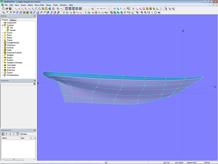
Model clipper-tangent_mcs.ms2 – 9 B-spline mcs each support the C-spline Lofted Surfaces topside and hull. Vertex curves connect corresponding control points.
In order to make the chine in the stern between the C-spline Lofted Surfaces topside and hull run out to the front, the mcs in this area must meet tangentially to each other. For this purpose, a Bead is created on each of the front mcs for surface hull at the start of the curve (t = 0), on which a Tangent Point depends. The mcs of topside are now defined with cp1 and these two points. The Tangent Point hardwires the tangential joint of the mcs of topside and hull.
The aft mcs are arranged like cant frames to form the rounded stern. The last three mcs of topside are Lines (mc7_top, mc8_top, mc9_top). The mid cps on these mcs required for the vertex curve vl2_top are Beads with the parameter value t = 0.5.
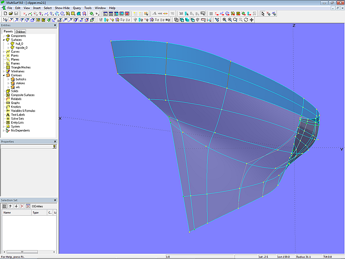
Model clipper-tangent_mcs.ms2 – Two-Surface approach. The stern mcs are arranged as cant frames.
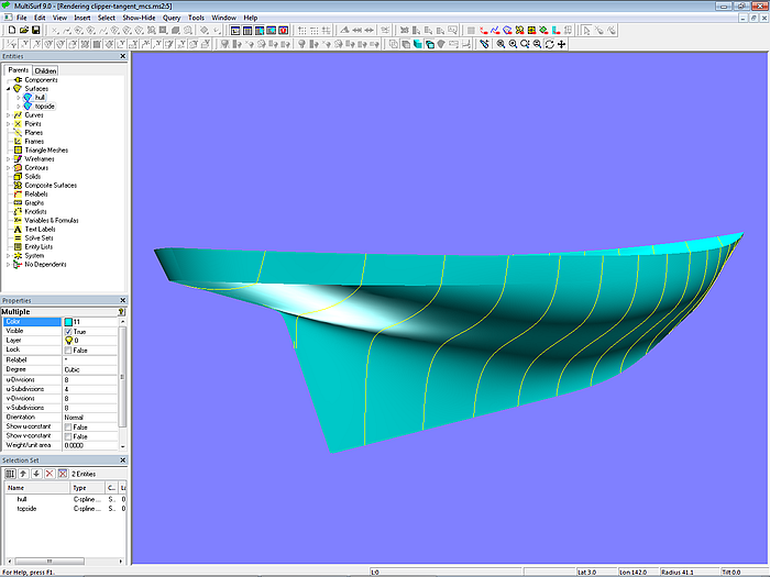
Model clipper-tangent_mcs.ms2 –Two-Surface approach
3.1.2 One-Surface approach – master curves connected to PolyCurves
In model clipper-polycurve_mcs.ms2 first a base surface without a chine is created (C-spline Lofted Surface hull_fair). The vertex curve method is used for it. In this way one obtains a fair hull with master curves whose control points are regularly arranged in the longitudinal direction and therefore have a regular parameter distribution. If inharmonious u-parameter curves later appear on the actual surface hull_w_chine, nothing needs to be changed in the mcs taken over from hull_fair, only the parameter distribution of the PolyCurves needs to be modified.
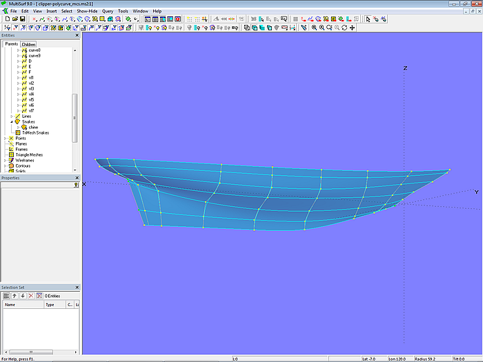
Model clipper-polycurve_mcs.ms2 – mcs and vertex curves of the C-spline Lofted Surface hull_fair
Next mcs with break points are added in the aftship for topside and hull surface, which are then connected to PolyCurves (mc7_poly, mc8_poly, mc9_poly). With the front mcs and the PolyCurves the actual hull surface is defined with a vanishing chine (C-spline Lofted Surface hull_w_chine).
The end t-value for mc7_poly, mc8_poly and mc9_poly must be chosen so that the UVSnake chine runs smoothly. It must be the same on all the PolyCurves.
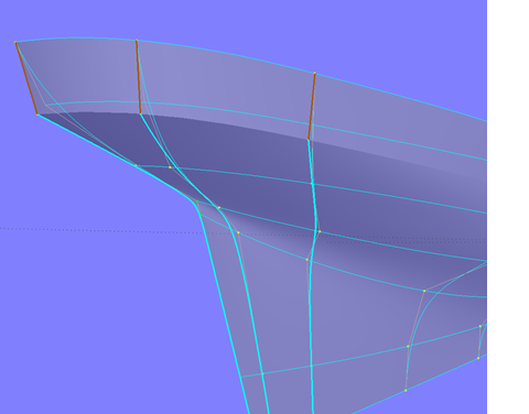
Model clipper-polycurve_mcs.ms2 – segments the stern master curves
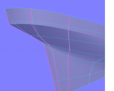
Model clipper-polycurve_mcs.ms2 – segments combined to PolyCurves
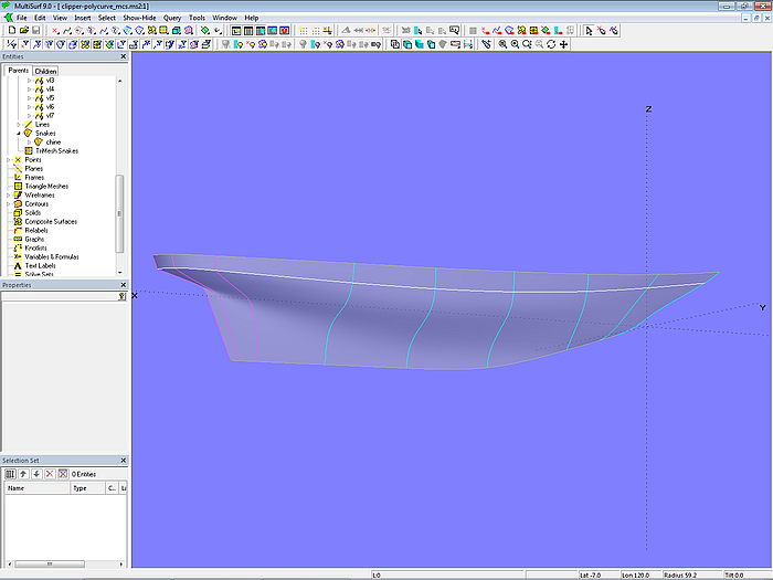
Model clipper-polycurve_mcs.ms2 – mcs running from top to bottom edge of the hull support the C-spline Lofted Surface hull_w_chine. The front mcs are B-spline Curves, the three aft mcs are PolyCurves.
If we look at the u parameter curves, we notice a somewhat inharmonic run in the lower stern area.
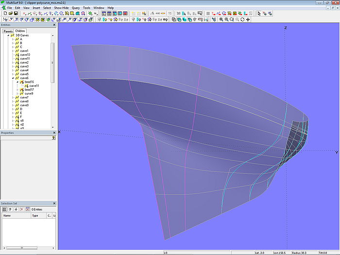
Model clipper-polycurve_mcs.ms2 – inharmonious run of the lower u-parameter curves in the stern
To correct this, the parameter distribution of mc7_bot is relabeled with the SubCurve mc7_hull_sub and the inner Beads bead1 and bead2.
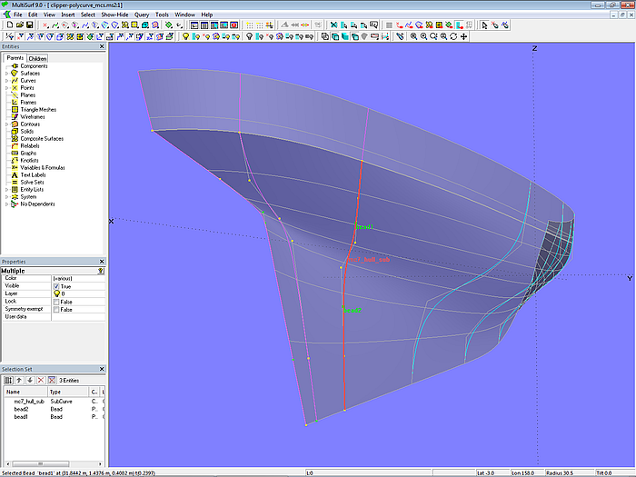
Model clipper-polycurve_mcs.ms2 – u-parameter curves made fair with SubCurve relabel
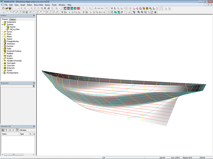
Model clipper-polycurve_mcs.ms2
3.2 Powerboat hull – foreship with vanishing chine
Another example is the hull of a motorboat. Here the partial length chine is to compensate for station flare in the forebody.
3.1.1 Two-Surface approach – master curves tangentially connected
In model powerboat-tangent_mcs.ms2 the hull is created using the Two-Surface approach. This means that the chine in the forebody extends over the entire length and divides the hull into the two C-spline Lofted Surfaces topside and hull. Both surfaces have the same number of mcs, which are tangentially connected with the help of Tangent Points except for the bow area.
When constructing the model in this way, the vertex curve method can be used for fairing (see appendix). The chine curve is also a vertex curve (C-spline Curve vl3_chine). Its shape is directly determined by the corresponding cps.
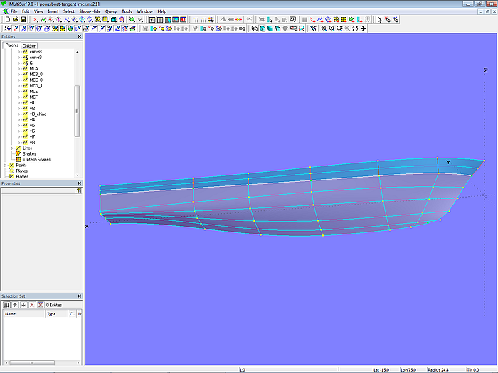
Model powerboat-tangent_mcs.ms2 – master curves and vertex curves of the C-spline Lofted Surfaces topside and hull
3.1.2 One-Surface approach – master curves connected to PolyCurves
In model powerboat-polycurve_mcs.ms2 the hull is modeled using the One-Surface approach. Mcs running from the top to the bottom edge of the hull support the surface. The mcs in the bow area are PolyCurves, the other mcs are B-spline Curves.
Here too, the starting point is a base surface without a chine, the C-spline Lofted Surface hull_fair. All its mcs are B-spline Curves with the same number of cps and the same degree. That's why the vertex curve method is used for fairing.
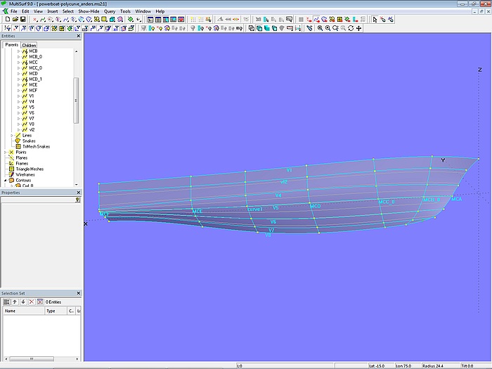
Model powerboat-polycurve_mcs – smooth base surface hull_fair with continuous mcs and vertex curves
In the foreship, mcs with breaks are now added for the upper and lower hull surface. These mcs are then connected to PolyCurves (mc2_poly, mc3_poly).
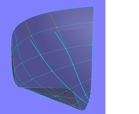
Model powerboat-polycurve_mcs – segments of the foreship master curves
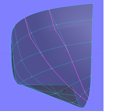
Model powerboat-polycurve_mcs – segments combined to PolyCurves
With the PolyCurves in the bow area and the aft mcs the actual hull surface with vanishing chine is created (C-spline Lofted Surface hull_w_chine). The end t-value for mc2_poly and mc3_poly must be chosen appropriately so that the UVSnake chine runs smoothly. The value must be the same on both PolyCurves.
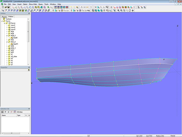
Model powerboat-polycurve_mcs.ms2 – the mcs of the C-spline Lofted Surface hull_w_chine in the bow area are PolyCurves.
As in the models sailboat-polycurve_mcs-1.ms2 and clipper-polycurve_mcs.ms2, the shape of the u-parameter curves must be checked. The easiest way to fix unfairness is to relabel mc2_bot and mc3_bot with SubCurves and use them for the PolyCurve segments. This construction is selected for the model powerboat-polycurve_mcs.ms2.
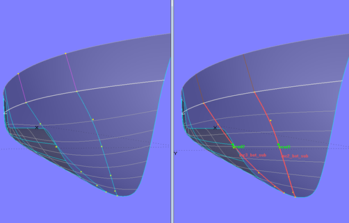
Model powerboat-polycurve_mcs.ms2 – left: irregular shape of the u-parameter curves; right: regular shape of the u-parameter curves by SubCurve relabeling
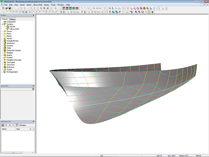
Model powerboat-polycurve_mcs.ms2
4 Summary
This tutorial shows methods how to create hull shapes with a series of stations showing a break point.
The Two-Surface approach – separate mcs
Mcs in the smooth portion of the hull touch tangentially. Regular course of the parameter curves using the vertex curve method. Chine curve equals vertex curve.
The Two-Surface approach – split mcs
Continuous mcs in the smooth part of the hull are divided into SubCurves. Mcs in the chine area must be relabeled to get fair parameter curves.
The One-Surface approach – continuous mcs and PolyCurves
Continuous mcs in the smooth part of the hull and PolyCurves in the chine area. PolyCurve segments must be relabeled to achieve fair parameter curves.
Which method is most appropriate for a hull with a vanishing chine depends on how large the proportion of the smooth hull surface is compared to the area with chine.
In the examples of the classic yacht and the powerboat, the chine curve runs at a relatively short distance from the top edge of the hull. The upper surface strip is narrow compared to the lower one, and the chine area is relatively small. The chine is more or less a local shape feature; the larger portion of the hull surface shows smooth stations. Then the One-Surface approach (continuous mcs and PolyCurves) is obvious. Starting from a smooth basic hull, the hull is “pushed” outwards into the desired shape using PolyCurves in the chine area.
If the Two-Surface approach with separate mcs is used for such a hull shape (relatively small chine area), the mcs for the narrow upper surface are relatively short. And since the mcs for this area have to be defined with at least 3 cps, they are close to each other. Although mcs that belong together are firmly tangentially connected with the help of Tangent Points, if something is changed in the mcs for the wider lower surface, the cps have to be re-positioned. Appropriate fine adjustment is required.
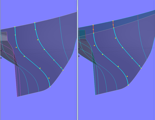
Control point distribution – left: continuous mcs; right: tangentially connected mcs
If for a hull shape with chine close to the top edge the Two-Surface approach with SubCurves of continuous mcs is used, then their cps can be distributed more evenly along the curve.
In the example of the sailboat hull, the distance of the chine curve from the top edge of the hull is greater, it is closer to the center of the stations. Then both variants of the Two-Surface approach are suitable.
5 Appendix – the Vertex Curve Method
The task when modeling a hull is not only to create a surface in the desired shape, the surface must also be smooth, it must be fair. Similar to an actual hull made of clinker, carvel or strip construction with its harmoniously running planks, a C-spline Lofted Surface is smooth if its generating lofting curves (its "planks") are fair.
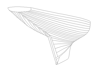
The run of the lofting curves is displayed if “Show u-constant” is set to “True” in the properties of a lofted surface in the Properties Manager. Then the series of lofting curves specified with the u-Divisions property is displayed. These curves are also called u-parameter curves of the surface.
The shape of the u-parameter curves depends on the parameterization of the master curves. If the mcs are equal in type and number of cps and if the cps are arranged harmoniously, the u-parameter curves are also regular.
A simple way to arrange cps harmoniously is to connect all corresponding cps of the mcs with C-spline Curves. These curves are called vertex curves. They show how the position of corresponding cps changes from bow to stern. Vertex curves are guiding curves for fairing a C-spline Lofted Surface. If they run in a harmonious, regular manner, the surface is smooth.
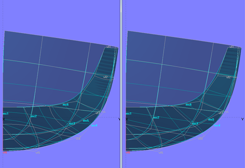
With a C-spline Lofted Surface, there is a close relation between the run of u-parameter curves and vertex curves.
One of the requirements of the vertex curve method - all mcs must have the same number of cps – forces, that the mc with the most complicated shape determines the necessary number of cps. Although other mcs could be defined with fewer points, the required higher number must be used.
This disadvantage is more than outweighed by the ability to use the vertex curve method to quickly and visually control the fairness of a C-spline Lofted Suface.
The modeling task therefore has two sides – one has to arrange the cps on all mCs in such a way that the desired hull shape results and at the same time the vertex curves take on a fair run.
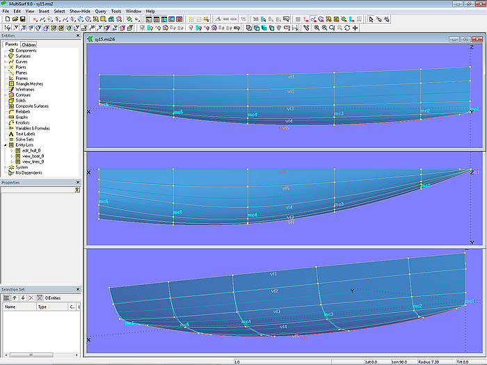
Vertex curves as fairing aid
It should be emphasized that irregular u-parameter curves are not necessarily an indication of surface unfairness. Imagine a smooth hull of white color with longitudinal curves drawn on it with a black pen. No matter how crooked they may be, the hull remains smooth.
However, modeling hulls using the vertex curve method is much easier and faster than trying with dissimilar mcs (because different in type, degree or number of cps) to achieve regular u-parameter curves by relabeling, or by constantly checking whether the surface is still smooth even though the u-parameter curves are not fair.
======================================================================================